
Confidence travels with assumptions
A hyperspectral classifier can be accurate on familiar samples and confidently wrong in a new region, season or acquisition batch. A probability of 0.95 is an output of a model, not a certificate that the spectrum resembles its training data. Before using that number to automate a decision, ask which observations, labels and operating conditions made it meaningful.
Domain shift concerns a change in the joint distribution of inputs and labels between a reference setting and the setting where predictions are used. Uncertainty concerns what the model communicates about its predictions. They interact, but neither is a substitute for the other. A changed input distribution need not make every prediction wrong, and an unchanged input histogram does not prove that the old label relationship still holds.
This guide builds a deliberately small counterexample. The interactive lab uses an original analytic score model and generated labels, with separate calibration, policy-validation and evaluation samples. Every displayed probability and metric is computed in the browser. There are no measured spectra, hidden training runs or real-world accuracy claims.
Name the distribution that changed
Let X denote the model input, Y the reference class, s the source distribution and t the target distribution. Under pure covariate shift, Pₜ(X) differs from Pₛ(X), while Pₜ(Y|X) = Pₛ(Y|X). Sugiyama and colleagues use this definition in their work on importance-weighted cross-validation. The unchanged conditional is an assumption to justify, not something established by noticing different spectral histograms. [1]
Under label shift, Pₜ(Y) changes while Pₜ(X|Y) remains fixed. Lipton and colleagues explicitly study this factorisation. A crop class becoming more common is a possible motivation, but does not establish pure label shift: its within-class spectra may also change with season, moisture or acquisition conditions. [2]
Here, conditional or concept shift means that P(Y|X) changes. Terminology varies across the literature, so write the distributional statement beside the name; Moreno-Torres and colleagues discuss this ambiguity. A different labelling rule or a changed relationship between a measured feature and the target can produce such a change. Several factors can move together, so these definitions are useful controlled cases rather than mutually exclusive descriptions of every field campaign. [3]
| Shift | What changes | What is held fixed in the pure case |
|---|---|---|
| Covariate | P(X) | P(Y|X) |
| Label / prior | P(Y) | P(X|Y) |
| Conditional / concept | P(Y|X) | P(X) need not be fixed; it is fixed in this toy |
| Unseen class | The supported label set expands | No closed-set coverage assumption |
Connect the statistics to HSI
For HSI, start with an acquisition-and-sampling ledger: sensor and spectral response, wavelength support, radiometric units, illumination, atmosphere, view geometry, spatial footprint, location, date, sample preparation and reference-label procedure. Differences in any of these are reasons to investigate transfer. They are not automatically proof of a particular statistical shift type.
Tuia, Persello and Bruzzone discuss remote-sensing domain adaptation in terms of the representativeness of training samples and differences in acquisition conditions, atmosphere and observed objects. Their review covers adaptation strategies for high-spatial- and high-spectral-resolution data. It supports treating transfer as an experimental question rather than assuming that a model is portable because its input arrays have the same shape. [4]
The same reasoning applies to laboratory batches. Imagine a hypothetical material classifier whose development samples all come from one preparation batch. New batches could differ in grinding, moisture, packing or measurement day. Holding out pixels from the original samples tests a much narrower claim than holding out physical samples and entire batches. This is an illustrative design example, not a claim about any particular unpublished experiment.
Preprocessing can reduce known measurement discrepancies, but it does not establish that class relationships are invariant. The preprocessing guide covers transformations; here the question is what evidence supports carrying a prediction rule into a new setting.
Interactive learning lab · synthetic data
Does source confidence survive a new domain?
Change only the evaluation setting. The temperature is fitted on 1,600 source calibration cases; the acceptance threshold is selected on 1,600 separate source validation cases. The 1,600 evaluation labels only measure the result.
Independent source-like samples: the same generating distribution, with different pseudorandom labels.
- Accuracy
- 76.8%
- Mean confidence
- 77.5%
- Top-class ECE
- 0.007
- Brier score (sum)
- 0.332
- Accepted coverage
- 47.7%
- Accepted error
- 11.5%
Source-like evaluation. Calibration temperature T = 1.945. Validation-selected confidence threshold 88.7%; validation coverage 49.3% and accepted error 14.5%. Evaluation accepts 763 of 1600 cases. This is an empirical toy policy, not an error guarantee.
● Source validation■ Evaluation
Class-1 ECE: 0.016. Mean predicted class-1 probability: 50.0%; observed class-1 frequency: 48.6%. Top-class ECE can hide class-specific miscalibration. These are evaluation diagnostics, never calibration inputs.
Policy controls and metric definitions
ECE is the count-weighted absolute bin gap. Top-class and class-1 ECE answer different questions. The Brier score sums squared probability errors across classes (range 0–2, lower is better). A zero-probability third-class slot permits scoring unseen-class cases. No cases accepted means accepted error is undefined. No field-performance or error guarantee is implied.
Evaluation reliability counts and values
| Confidence bin | Count | Mean confidence | Correctness |
|---|---|---|---|
| 0–10% | 0 | No samples | No samples |
| 10–20% | 0 | No samples | No samples |
| 20–30% | 0 | No samples | No samples |
| 30–40% | 0 | No samples | No samples |
| 40–50% | 0 | No samples | No samples |
| 50–60% | 0 | No samples | No samples |
| 60–70% | 837 | 67.3% | 66.1% |
| 70–80% | 0 | No samples | No samples |
| 80–90% | 763 | 88.7% | 88.5% |
| 90–100% inclusive | 0 | No samples | No samples |
Risk–coverage values
| Split | Threshold | Accepted | Coverage | Error |
|---|---|---|---|---|
| Validation | 88.7% | 788 | 49.3% | 14.5% |
| Validation | 67.3% | 1600 | 100.0% | 24.6% |
| Evaluation | 88.7% | 763 | 47.7% | 11.5% |
| Evaluation | 67.3% | 1600 | 100.0% | 23.3% |
Static default view. JavaScript enables the controls.
Calibration is a population statement
For top-class confidence, calibration asks whether predictions given similar confidence are correct at a corresponding frequency on a specified population. A group of predictions around 80% confidence should be correct about 80% of the time under that interpretation. It does not say which individual cases are wrong, and it is weaker than validating every class probability or every subgroup.
Guo and colleagues evaluate neural-network calibration and describe temperature scaling: divide logits by a positive fitted temperature before converting them to probabilities. The temperature is chosen using held-out labelled data. Their favourable empirical results on studied datasets are not a guarantee for a new HSI sensor, an unseen class or arbitrary distribution shift. [5]
A positive common temperature preserves the winning class. It can change probability quality without changing accuracy. In this lab it also preserves confidence ranking because there are only two scored classes and confidence is monotone in the absolute logit. That ranking property should not be assumed for every multiclass system.
Ovadia and colleagues directly evaluate predictive uncertainty under dataset shift. Their benchmark shows that conventional post-hoc calibration and other uncertainty methods can deteriorate as the distribution changes. The relevant lesson is to evaluate uncertainty on the intended shifts; the paper does not supply an HSI-specific performance guarantee. [6]
Read the lab as a controlled counterexample
The source generator chooses one of four scalar feature values: −2, −0.7, 0.7 or 2, initially with equal probability. A class-1 label is drawn with probability sigmoid(x). The synthetic classifier uses logit 2x, making its probabilities too sharp for the generating conditional. The feature is dimensionless; it is not a wavelength, reflectance value or fitted spectral embedding.
Three sets contain 1,600 cases each, with fixed seeds 1001, 2002 and 3003. The first fits a temperature by minimising binary negative log likelihood over T ∈ [0.2, 5]. The second selects an abstention threshold. The third reports evaluation results. The records have distinct IDs, although discrete feature values deliberately repeat across sets. No training claim is made: the score rule is specified by hand.
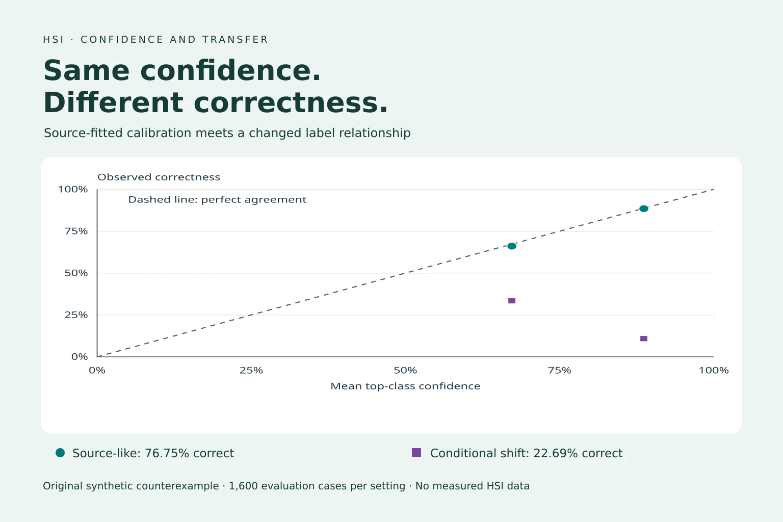
With the default source-like evaluation, fitting the temperature gives T ≈ 1.945. Accuracy remains 76.75%; top-class ECE changes from about 0.120 uncorrected to 0.007 corrected, and the sum-form Brier score changes from about 0.362 to 0.332. These are deterministic results for these generated samples, not estimates of HSI performance.
Now select covariate shift at full severity. The feature weights become 0.1, 0.4, 0.4 and 0.1, favouring ambiguous cases while preserving the label conditional. Accuracy falls to about 70.81%, but corrected ECE remains about 0.007. Exact conditional probabilities would remain calibrated under this particular shift. A worse task mix can reduce accuracy without making probabilities misleading.
One small ECE can hide the wrong probabilities
The label-shift preset raises the population class-1 prior from 0.50 to 0.85 while preserving P(X|Y). Its target feature weights and label probabilities are derived using Bayes’ rule. This differs from simply forcing extra positive labels into the same feature distribution, which would usually change P(X|Y).
At full label shift, this symmetric toy has corrected top-class ECE of about 0.007, but class-1 ECE of about 0.225. Mean predicted class-1 probability is about 63.05%, while the observed class-1 frequency is 85.50%. Combining predictions of opposite classes in the same top-confidence bin can conceal errors in individual class probabilities. This constructed example is why the lab shows a separate class-1 diagnostic.
Conditional shift keeps the same feature distribution and increasingly reverses the label probabilities. At full severity, corrected mean confidence stays about 77.47% while accuracy falls to about 22.69%. Monitoring inputs alone cannot distinguish this generator from its source distribution. Labels, or other valid evidence about the changed relationship, are needed.
The sensor-offset preset adds up to 1.5 to the observed feature while retaining labels generated from the latent feature. It is an acquisition-style perturbation, not a simulated hyperspectral instrument or a pure-covariate-shift claim. The unseen-class preset instead inserts up to 35% novel cases at x = 3.4. The two-class model confidently assigns them to a known class, illustrating why low uncertainty is not an out-of-distribution detector by itself.
Read reliability bins with their counts
Each reliability point shows the mean top-class confidence and observed correctness within a bin. The dashed diagonal denotes equality. Bins are left-closed and right-open, except the last bin includes 1. Empty bins have no point and are labelled “No samples” in the table; they are not observations of zero accuracy. The lab offers 5, 10 or 15 equal-width bins.
Expected calibration error here is the count-weighted mean absolute difference between bin accuracy and mean confidence: ECE = Σᵦ (nᵦ/n)|accuracyᵦ − confidenceᵦ|. It is a finite-sample, bin-dependent diagnostic. Altering the bins can alter its value, and a low aggregate value can hide class-, region- or batch-specific problems. The displayed class-1 ECE bins P(Y = 1) against the indicator that the reference label is 1.
The Brier score uses the full probability vector: mean over cases of Σₖ(pₖ − 1{Y = k})². We use the sum over classes, not an average across classes, giving a 0–2 range with lower values better. It measures overall probabilistic error, not calibration alone. For consistent scoring across presets, every vector has three entries; the unmodelled class always receives probability zero. Known-class cases therefore reproduce the two-class sum convention.
Both charts use fixed 0–1 axes across presets. The points and line segments summarise a small discrete score model, so their sparseness is intentional. No error bars are shown: these are repeatable teaching samples, not a field-study uncertainty interval. Real correlated imagery needs an uncertainty analysis at a defensible independent sampling unit.
Abstention is a policy with a cost
Selective prediction allows a system to decline some cases. Coverage is the fraction accepted; selective risk is the error rate among accepted cases. El-Yaniv and Wiener formalise this risk–coverage trade-off in selective classification. The possibility of rejecting predictions is useful only if the remaining errors and the cost of declined cases are acceptable for the application. [7]
The lab chooses the lowest confidence threshold that achieves the requested empirical error target on the separate source policy-validation set, while accepting at least 30 validation cases. This maximises validation coverage among its candidate thresholds. If none qualifies, the policy accepts nothing and the accepted error rate is “Not defined”, never zero. A minimum count of 30 is a teaching choice, not a statistical guarantee.
The default 20% target selects a threshold of about 88.66% after correction. Applied to source-like evaluation it accepts about 47.69% of cases with 11.53% error among them. Applied unchanged to full conditional shift, it accepts the same fraction but incurs about 89.12% error among accepted cases. High confidence now ranks many wrong predictions above correct ones.
The evaluation risk–coverage curve is diagnostic only: its labels do not choose the policy. Tuning a threshold after inspecting these evaluation labels would turn that set into development data. A production review must also count the workload, delays and outcomes for declined cases. Lower coverage can shift work onto human review or exclude particular classes and locations.
Match the holdout to the generalisation claim
Liang and colleagues examine evaluation design for spectral–spatial HSI classification, including the problems that arise when training and test samples are randomly drawn from the same image. Nearby samples and overlapping spatial context can make the resulting evaluation less independent than the nominal pixel count suggests. [8]
A held-out pixel, a new physical specimen, a different field, a new geographic region and a new season answer different questions. Choose the grouping unit before fitting a model or calibrator. If the intended claim is geographic transfer, retain whole target regions for final evaluation; an independent pixel sample from the source region cannot establish that claim. The spatial-splits guide explains the separation problem in more detail.
Keep model training, model selection, calibration and policy selection distinguishable. With limited data, a carefully designed nested or cross-fitting procedure may reuse information more efficiently, but the final evaluation must remain outside the decisions it measures. Fit feature scaling, dimensionality reduction and other learned transformations inside the relevant development split.
Report accuracy, probability scores, reliability and acceptance rates by relevant domain and class as well as overall. State how many independent regions, dates or batches were observed, not only how many pixels. If uncertainty intervals are needed, resampling should respect the dependence structure; millions of adjacent pixels do not create millions of independent deployment trials.
Build an operating envelope
Before deployment, write down where the model has evidence: supported sensors and bands, units, acquisition conditions, class definitions, locations, seasons and sample types. Record what lies outside that evidence and what happens there. An abstention path needs an owner and a practical next action, such as another measurement or expert review.
A useful transfer experiment compares a fixed source model with clearly declared adaptation options. If target examples are used for calibration, feature alignment or fine-tuning, disclose that access and reserve independent target evaluation data. Domain adaptation uses target-domain information under a stated protocol; domain generalisation aims to handle unseen domains without adapting to their data at deployment.
Collect justified monitoring signals: changes in acquisition metadata, missing bands, input distributions, predicted class frequencies, confidence distributions, acceptance rates and subsequently verified errors. None alone establishes safe transfer. A stable confidence histogram is particularly weak evidence in the conditional-shift counterexample.
The practical conclusion is modest but useful: confidence needs a population, calibration needs held-out evidence, and abstention needs a validation protocol and a cost model. Validate these together at the scale of the claim. A well-calibrated source model is a starting point for a transfer study, not the end of one.
Frequently asked questions
Does calibrated confidence detect out-of-distribution spectra?
Not by itself. Calibration describes a relationship on an evaluated population. A closed-set classifier can confidently assign an unseen class to a known class.
Does every domain shift make calibration worse?
No. Under pure covariate shift, an exact unchanged conditional-probability model remains calibrated even if accuracy and coverage change. Real fitted models may not satisfy that condition.
Can low ECE hide problems?
Yes. Binning and aggregation can conceal class- or domain-specific errors. The lab’s label-shift case has low top-class ECE alongside much larger class-1 ECE.
Can I tune the confidence threshold on the test set?
Doing so makes the test set part of development. Choose the rule on validation data and report its result on a separate evaluation set.
Does accepting no cases produce zero error?
No. Coverage is zero, but the error rate among accepted cases is undefined because there are no accepted cases.
Is the toy a real hyperspectral benchmark?
No. It uses a scalar analytic score model and generated labels. Its role is to isolate statistical mechanisms, not estimate real HSI accuracy or sensor behaviour.
References and further reading
- Sugiyama, M., Krauledat, M. & Müller, K.-R. (2007). Covariate Shift Adaptation by Importance Weighted Cross Validation. JMLR 8, 985–1005.
- Lipton, Z. C., Wang, Y.-X. & Smola, A. J. (2018). Detecting and Correcting for Label Shift with Black Box Predictors. ICML, PMLR 80, 3122–3130.
- Moreno-Torres, J. G. et al. (2012). A unifying view on dataset shift in classification. Pattern Recognition 45(1), 521–530. DOI: 10.1016/j.patcog.2011.06.019.
- Tuia, D., Persello, C. & Bruzzone, L. Recent Advances in Domain Adaptation for the Classification of Remote Sensing Data. Author manuscript, arXiv:2104.07778.
- Guo, C., Pleiss, G., Sun, Y. & Weinberger, K. Q. (2017). On Calibration of Modern Neural Networks. ICML, PMLR 70, 1321–1330.
- Ovadia, Y. et al. (2019). Can You Trust Your Model’s Uncertainty? Evaluating Predictive Uncertainty Under Dataset Shift. NeurIPS 32.
- El-Yaniv, R. & Wiener, Y. (2010). On the Foundations of Noise-free Selective Classification. JMLR 11, 1605–1641.
- Liang, J., Zhou, J., Qian, Y., Wen, L., Bai, X. & Gao, Y. (2017). On the Sampling Strategy for Evaluation of Spectral-Spatial Methods in Hyperspectral Image Classification. IEEE TGRS 55(2), 862–880.
Reader feedback
Reads since 1 October 2026: at least 15 seconds with the article visible, counted once per browser per day. Reactions are anonymous and can be changed.
Loading reader feedback…
Discuss this article
Ask a technical question, challenge an assumption or share evidence from your own work.