
Start with a spectrum you can account for
Preprocessing should make a measurement easier to analyse without hiding what happened to it. A smooth curve is not proof of a better spectrum, and a standardised matrix is not proof of a fair experiment. This guide builds a small, testable Python workflow: validate the wavelength axis, flag unreliable bands, preserve gaps, choose a spectral transformation and fit learned transformations on training data only.
The input is an observation-by-band matrix. An observation may be an extracted pixel spectrum, an object-average spectrum or a bulk spectrometer reading. Those observations have different independence assumptions even when their arrays have the same shape. Keep the sample identifiers and acquisition metadata alongside the matrix.
The chickpea flour NIR guide explains the measurement and the distinction between a bulk spectrum and an image cube. The reflectance-calibration guide covers dark and panel references. Here we begin after the measurement representation has been established. The operations below are general teaching examples, not a reconstruction of the chickpea paper’s selected preprocessing.
Check wavelengths, units and missing values first
Use an explicit spectral axis: X.shape = (n_observations, n_bands), paired with one wavelength per column. Convert the wavelength unit deliberately, for example from micrometres to nanometres. Require finite, positive, unique coordinates. If the file stores descending wavelengths, sort the coordinate array and apply exactly the same permutation to spectra, quality flags and other band metadata. Sorting only the labels silently attaches measurements to the wrong wavelengths.
Distinguish digital counts, fractional reflectance, percentage reflectance and pseudo-absorbance. Read a product’s scale factor, offset and no-data definition rather than guessing from its histogram. For example, NEON documents stored reflectance scaling and a separate data-ignore value. Apply that product’s conversion and mask rules before treating its numbers as physical values. A no-data sentinel is not a strong absorption feature. [1]
The downloadable functions intentionally reject non-finite inputs. The synthetic data are complete before a known band mask is applied; this makes every transformation auditable. For real missing observations, choose and record a policy before calling these functions. Do not replace NaNs with zero, silently drop different bands from each row, or fill a long missing interval and then describe the invented values as observations.
Sources: [1]
| Operation | Acts across | Learns from other observations? | Output / main caution |
|---|---|---|---|
| Fixed bad-band mask | Wavelength metadata | No, when independently specified | Retained bands; preserve physical gaps |
| Row min–max / z-score / SNV / L2 | Bands within one spectrum | No | Different invariants; denominator and amplitude trade-offs |
| MSC in this example | Row fitted to mean training spectrum | Yes: reference from training rows | Corrected signal; reject unstable reference/gain |
| Linear / quadratic detrending | Each contiguous run in one spectrum | No | Residual signal; may remove broad absorption structure |
| Moving average | Local bands within one valid run | No | Signal units; shorter edge windows |
| SG first derivative | Local wavelength neighbourhood | No, with fixed settings | Per nm; uniform spacing within each segment |
| StandardScaler | Observations for each band | Yes, training observations | Feature-scaled values; store train means/scales |
| PCA | Feature covariance structure | Yes, training observations | Component scores; fit inside each fold |
Flag bad bands with a reason, not a favourite wavelength list
A band mask should have a traceable reason: a product quality flag, saturation, a weak reference denominator, an independently characterised detector problem or a documented low-signal interval. Read the sensor and product metadata first. NEON’s processing tutorials provide a concrete example of using product bad-band windows rather than assuming every stored band is equally usable. [2]
The correct mask depends on the instrument, illumination, measurement geometry and processing level. An atmospheric absorption interval in an airborne product is not automatically an interval to remove from a laboratory material spectrum. A useful chemical feature can also be a deep absorption. Do not copy a wavelength exclusion list without checking what made those measurements unreliable.
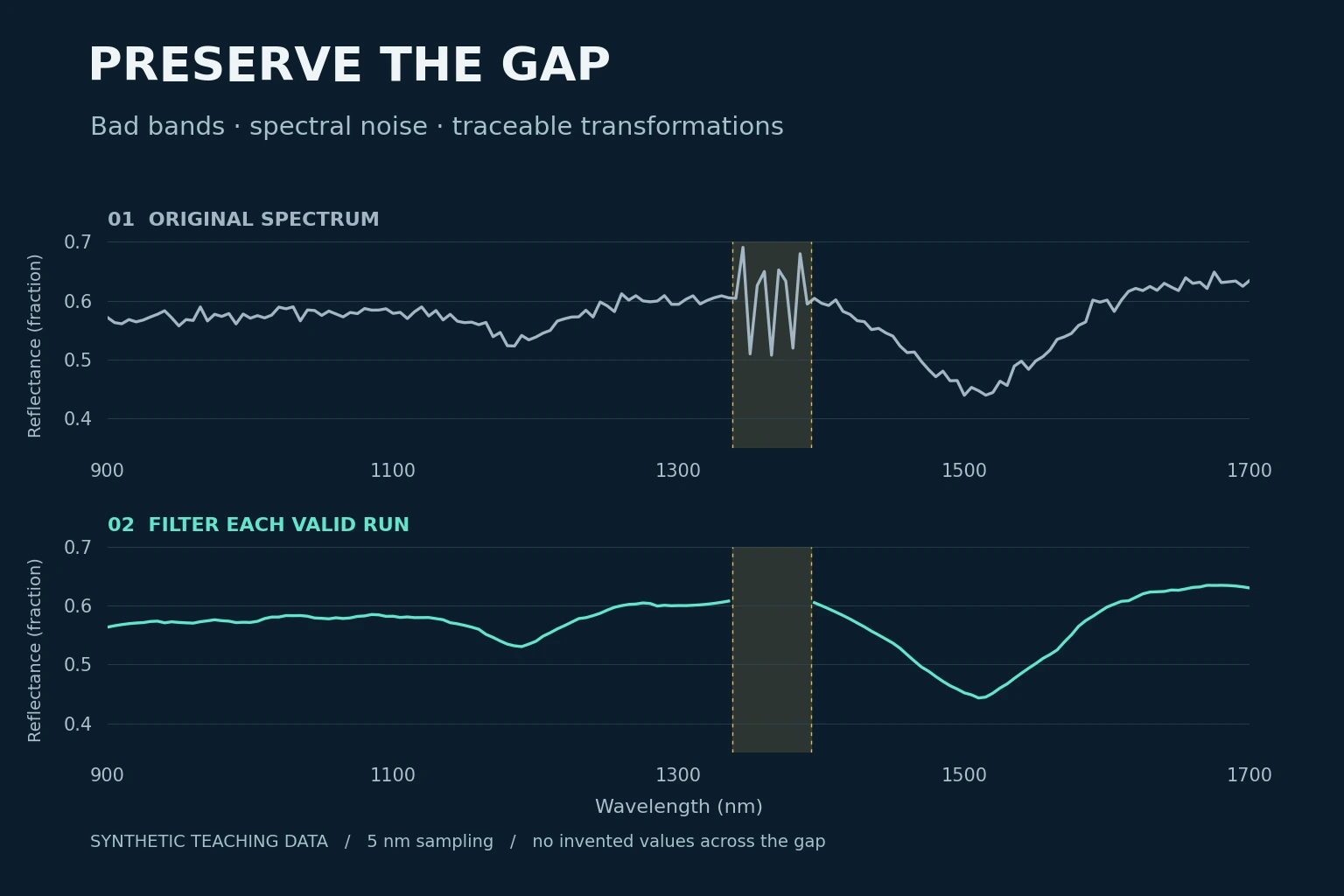
In this demonstration, 11 values from 1340 to 1390 nm are deliberately corrupted on a 900–1700 nm grid sampled every 5 nm. Their rejection is known from how the example was constructed. These values are illustrative, not a recommendation for your sensor. The playground lets you include them again to see how a filter can spread a corrupted value into its neighbours.
Sources: [2]
Spectra playground · synthetic data · CPU reproducible
Change the nuisance. Compare the recipe.
Try a practical set of common transformations, then inspect exactly what each one changes. There is no universal winner. All presets retain the deliberately corrupted 1340–1390 nm interval so you can test what happens when its mask is switched off.
Loading the self-contained synthetic example…
All values are synthetic: 161 wavelengths at 5 nm spacing, with 150 retained when masking is on. Training-fitted options use 44 fixed rows from 22 synthetic groups; current spectra do not update that reference. The supplied workflow deliberately requires the original complete uniform grid and finite inputs before masking. It never interpolates across the excluded interval.
What is each method allowed to change?
- Per-spectrum min–max sends that row’s retained minimum/maximum to 0/1 before filtering. It is not scikit-learn’s default per-feature MinMaxScaler.
- Per-spectrum z-score and SNV both centre a row; this playground distinguishes population SD (ddof=0) from sample SD (ddof=1).
- L2 divides each row by its Euclidean norm without centring it.
- MSC fits a gain and offset against a reference learned from the training rows, then applies (spectrum − offset) / gain.
- Per-band z-score uses training means and scales across observations, not the current spectrum’s own mean and scale.
- Detrending subtracts a line or quadratic separately in each valid run. It can remove genuine broad spectral structure.
- Savitzky–Golay fits degree-2 local polynomials. First and second derivatives have units per nm and per nm². Moving average uses an arithmetic mean and shorter windows at segment edges.
Order is fixed and visible: mask → detrend → normalise/scatter-correct → filter. Post-filter values need not retain a preceding normalisation’s range or variance. This is a useful subset, not every spectral preprocessing method.
Try three experiments
- Choose “Gain + offset”, then compare no normalisation, SNV and MSC. Watch the output units and the note explaining who supplies each reference.
- Choose “Turn up noise”, then compare moving average and SG using the same span. Inspect narrow structure and segment edges; a smoother line is not a performance score.
- Choose “Bend the baseline”, then compare linear and quadratic detrending. Notice that broad signal structure can disappear along with the nuisance.
Run the complete Python example
python -m pip install -r requirements.txt
python hsi_preprocessing.py --self-test
python hsi_preprocessing.py --preset scatter --normalisation msc \
  --operation derivative2 --window 11 --output example.csv
Exact command for the current settings:
Loading the current recipe…The download contains every function, fixed synthetic data generation, a CLI, unit tests and a self-contained executed notebook. It needs no GPU, account, private files or dataset download.
Download the complete Python bundle · Self-contained notebook
Removing columns does not close the physical gap
The original example has 161 samples and a constant 5 nm interval. After masking, 150 remain in two runs: 900–1335 nm and 1395–1700 nm. Those last and first retained wavelengths are 60 nm apart. Passing the compressed 150-column matrix to an ordinary Savitzky–Golay filter makes the two sides look adjacent in array space, even though they are not adjacent measurements.
The supplied implementation retains the full coordinate grid, filters each contiguous valid run separately and leaves excluded output values as NaN. The browser uses null for the same gaps and starts a new line segment after each one. No line connects the two sides of the missing interval. A deliberate test removes the columns and verifies that the uniform-spacing check raises an error.
For genuinely irregular sampling, a single average or median delta is insufficient. Either use a method that fits against the actual local wavelength coordinates, or justify resampling within measured, contiguous regions onto a uniform grid. Record that interpolation and its uncertainty; do not bridge a wide gap simply to satisfy a function signature. If a valid run is shorter than the requested window, the example stops with an error rather than borrowing samples across the gap.
Smooth locally, and report the physical span
Savitzky–Golay smoothing evaluates local polynomial fits rather than taking a plain moving average. The polynomial degree and window length control which variations the calculation can retain. Smoothing can reduce high-frequency variation, but it can also attenuate narrow structure; the smoothest-looking setting is not necessarily the most useful one. The method originates in Savitzky and Golay’s least-squares work. [5]
Our teaching configuration uses degree 2 and odd windows of 5, 11 or 21 bands. With 5 nm spacing, their first-to-last sample spans are 20, 50 and 100 nm respectively. These spans are not the instrument’s optical resolution. Report both the band count and wavelength span so another researcher can interpret the filter.
The Savitzky–Golay Python call uses axis=1 so that filtering runs along wavelengths, and mode="interp" for polynomial edge handling. The window must fit inside each segment. Edge estimates use one-sided information from that segment and deserve particular scrutiny; padding or edge fitting cannot recover observations beyond its boundary. Keep an unfiltered baseline in any model comparison. [3]
SNV changes each spectrum, not each wavelength column
Standard normal variate, or SNV, centres one spectrum across its retained bands and divides by that spectrum’s standard deviation. Barnes, Dhanoa and Lister introduced SNV in the context of diffuse-reflectance scatter effects. It is a possible representation, not a guarantee of removing every physical nuisance. [6]
This implementation uses zᵢⱼ = (xᵢⱼ − meanᵢ) / sᵢ, with sample standard deviation sᵢ calculated using ddof=1. After SNV alone, each retained row has mean zero and sample standard deviation one. A constant or nearly constant row has an unstable denominator and is rejected. State the convention: ddof=0 and ddof=1 give different numerical values.
The algebra explains the trade-off. For a positive gain a and wavelength-independent offset b, SNV(a·x + b) = SNV(x). Our tests verify that identity. Removing absolute amplitude can also remove information relevant to the target, so compare SNV with a physically meaningful unnormalised baseline rather than treating it as compulsory.
In the playground the order is fixed mask → optional detrending → selected normalisation or scatter correction → optional filter. Smoothing before SNV changes the standard deviation used in the normalisation; SNV before smoothing does not generally end with unit variance. The tests deliberately verify that these two orders differ. The choice of retained wavelength range also changes the row mean and variance, so keep it consistent between calibration and prediction.
Sources: [6]
Compare normalisations by their axis and invariants
“Normalise” is not a complete method description. Per-spectrum min–max subtracts that row’s retained minimum and divides by its retained range. Its pre-filter extrema become zero and one. The per-spectrum z-score option uses that row’s population standard deviation, ddof=0; SNV here uses sample standard deviation, ddof=1. With m retained bands, the SNV values equal the population z-scores multiplied by √((m−1)/m). The distinction is small for many bands, but it should be explicit.
L2 normalisation divides the retained row by its Euclidean norm without centring it. It removes a positive overall scale but does not remove an additive offset. Min–max and z-score alter both the location and scale. All can suppress physically meaningful amplitude differences. Their invariants apply immediately after normalisation, not necessarily after a later derivative or smoothing step. [13]
The per-band z-score option is different: it uses a mean and population standard deviation estimated across fixed training observations at each wavelength. It does not force the displayed spectrum to have mean zero or variance one. Likewise, scikit-learn’s default MinMaxScaler learns feature-wise extrema across observations; it is not the row-wise min–max calculation in this playground. Always identify the axis and fitted population. A derivative after per-band standardisation differentiates the feature-scaled curve, not the original reflectance. [7][14]
Zero or nearly zero denominators are handled explicitly. Constant rows cannot supply a useful SNV/z-score/range denominator, and a zero vector cannot supply an L2 norm. The teaching functions reject those cases. For a constant training feature, the feature-wise standardiser uses scale one after centring, matching the intended no-division-by-zero behaviour.
MSC needs a reference, and its source matters
Multiplicative scatter correction, or MSC, is associated with the multivariate scatter-correction approach introduced by Geladi, MacDougall and Martens. In this implementation, the reference r is the mean of the training spectra after the same mask and optional detrending. For each new spectrum x, least squares fits x ≈ a + b·r over the retained wavelengths, then returns (x − a)/b. This is an empirical correction against a stated reference, not a proof that every physical scattering effect has been separated. [12]
The browser reference is derived from 44 fixed observations belonging to 22 synthetic training groups. Current sample controls never refit it. Changing the mask or detrending switches to the corresponding precomputed training recipe. The Python transformer learns that reference inside fit, so cross-validation constructs a new reference from each training fold. Supplying test spectra while learning the reference would violate that evaluation boundary.
A flat reference or a near-zero fitted gain makes the correction unstable. The example rejects those cases and also rejects non-positive gains, which do not fit its intended positive-gain teaching model. On an exact synthetic x = a + b·r with positive b, its unit test recovers r. That verifies the arithmetic; it does not establish a predictive advantage over SNV on measured data.
Sources: [12]
Detrending and moving averages make different assumptions
Linear detrending subtracts a fitted straight line; quadratic detrending subtracts a fitted second-degree polynomial. The playground fits each spectrum within each contiguous valid run, using centred and scaled wavelength coordinates for numerical conditioning. A broad absorption feature can influence that polynomial, so baseline removal can also remove real signal. Independent fits on either side of a gap can have different offsets; they are never joined as if the missing region had been measured. [15]
A centred moving average uses equal weights in its local window. Here its window shrinks at segment boundaries rather than padding, wrapping or crossing the missing interval. Its edge behaviour therefore differs from the polynomial edge estimates used by Savitzky–Golay. The test suite verifies those exact edge means. The displayed span is the nominal full window; fewer points are used at the edges.
The playground deliberately fixes a visible order: mask → detrend → normalise/scatter-correct → filter. Detrending before a normalisation changes its denominator or reference; smoothing before normalisation produces a different recipe. There is no order-independent “clean spectrum”. Validate the whole recipe, not just each named step in isolation.
Although row-wise normalisation itself can be defined on irregular wavelength coordinates, this combined runnable workflow intentionally requires a complete uniform input grid before masking. It stops on irregular or compressed gapped inputs. A coordinate-aware irregular-grid implementation is a separate modelling choice, not something a convenient mean spacing can repair.
Derivatives must be per wavelength, not per array index
A derivative describes local change with wavelength. For fractional reflectance R sampled in nm, the first derivative is dR/dλ in reflectance fraction per nm. A first derivative of SNV values is in normalised units per nm. The second derivative measures change in that slope and has units per nm². None of these derivative outputs should be labelled simply reflectance.
SciPy’s delta parameter sets sample spacing for derivative calculations. Leaving delta=1 on a 5 nm grid gives a derivative per sample, numerically five times the per-nm result. Our call sets delta to the validated spacing and deriv=1 directly; it does not first smooth and then apply the same derivative filter a second time. [3]
A useful unit test supplies a known quadratic curve and checks the analytical first derivative, including each segment’s edges. Another checks the unit conversion: the numerical first derivative per micrometre is 1,000 times the derivative per nanometre; the second derivative changes by 1,000,000. These checks catch unit and sign errors without pretending that a synthetic curve establishes real-world prediction accuracy.
Differentiation emphasises rapid changes and can magnify measurement noise. A constant offset disappears mathematically, but a changing baseline does not necessarily disappear. Inspect the derivative alongside the input, with its own labelled axis, and select its configuration using the intended validation design.
Sources: [3]
Keep learned scaling and PCA inside the training pipeline
SNV works within one row. StandardScaler instead estimates a mean and scale for each feature across training observations, then applies those stored values to other rows. The directions are different. StandardScaler also uses a population-style variance convention, whereas the SNV implementation here explicitly uses sample standard deviation. [7]
PCA learns a feature-space basis from its fitted observations. It centres its input but does not automatically standardise every feature to unit variance. Scaling before PCA therefore changes the problem PCA solves. Unit-variance scaling can give a noisy, low-variance band more influence, so the mask and the modelling purpose still matter. [8]
Fit learned scaling, imputation, feature selection and PCA on training observations only. A scikit-learn Pipeline keeps these operations with the estimator so each cross-validation fit learns its own transformations. Transform held-out data with the fitted objects; never refit them on the held-out set. [9][10]
The downloadable example places the fixed spectral preprocessor, StandardScaler, PCA and a small ridge regressor in one pipeline. Its synthetic target is a dimensionless curve-generation parameter. The example demonstrates plumbing and checks fitted statistics, not a compositional calibration, spectral unmixing model or accuracy benchmark.
Split independent units before choosing the recipe
An HSI cube can contain many strongly related pixels. If the intended claim is performance on new specimens, fields or acquisitions, define the split at that unit. Keep repeat scans of one sample together. The example creates two observations per synthetic sample and uses a grouped split; it also tests a grouped cross-validation pipeline. [11]
Fixed sensor-quality metadata and a per-row formula do not estimate population statistics. However, selecting a mask, SNV choice, derivative order or window because it improves test performance still leaks information through model selection. Choose those options on training/validation data, or inside an inner validation loop, and reserve the final test for the stated evaluation.
Preserve row identifiers, group identifiers and the wavelength schema when reshaping a cube into a table. Split design is a scientific decision, not an incidental call to reshape. A train-only scaler cannot repair an evaluation where nearly identical observations already occur on both sides.
Use controlled nuisances to ask a better question
Choose “Quiet signal”, “Turn up noise”, “Gain + offset”, “Bend the baseline” or “Mixed effects”. These presets only alter the synthetic input; they do not select a supposedly winning method. Expand the fine controls to adjust gain, additive offset, fixed-seed noise amplitude and quadratic curvature. The deliberately corrupted interval remains present in every preset so the band-mask lesson remains visible.
Try the gain/offset preset with L2, SNV and MSC and explain why their responses differ. Try the noisy preset with moving average and Savitzky–Golay at the same nominal span, then inspect a feature and a segment edge. Try curvature with both detrending choices and ask what genuine broad structure was removed along with the nuisance.
The two panels share their scale only when their units are comparable. A normalised or differentiated result has a separate labelled axis; a visually larger or smoother trace is not a score. Read the method’s fitting note, inspect a wavelength with the keyboard-accessible slider and download the actual displayed values. This is a practical, testable subset of preprocessing methods, not an exhaustive catalogue or a substitute for measured validation.
Run the CPU example and inspect what was tested
Download the notebook and Python bundle, then run python -m unittest -v test_preprocessing.py from the extracted folder. Run python hsi_preprocessing.py for the complete grouped training example. The self-contained notebook includes every function and walks through the same operations with printed checks and an intentional gap error. The script accepts named method/preset options and writes a CSV plus recipe metadata when an output path is requested; run python hsi_preprocessing.py --help for all switches. NumPy, SciPy and scikit-learn are the only numerical dependencies; no GPU, credentials or dataset download is needed.
The browser playground uses coefficients generated by SciPy for its fixed degree, window choices and grid. Its implementation is compared with 630 Python reference recipes: mask on/off, three detrending settings, seven normalisation choices including none, five filtering choices including none, and three windows, exercised on distinct synthetic spectra and nuisance settings. Agreement checks include edge values and explicit gaps. These are numerical consistency tests, not evidence that any preprocessing option improves a real application.
The 25 Python tests check sorting and units, invalid coordinates, missing-data rejection, masked corruption isolation, row-normalisation invariants, MSC reference/slope guards, polynomial detrending, first/second derivative accuracy, moving-average edges, too-short segments, CLI output, pipeline cloning and fold-local scaler/PCA/MSC statistics. Preserve the source, random seed, versions and test output with any adapted workflow so later changes remain reviewable.
A short checklist before trusting the transformed matrix
Keep the original measurement and an auditable transformed copy. A useful preprocessing record should let someone answer each of the following without reverse-engineering the notebook.
- What does a row represent, and which observations must remain in the same split?
- What are the signal and wavelength units, and which product scale/no-data rules were applied?
- Which bands were excluded, why, and were every spectrum and metadata field reordered together?
- Did any filter or plotted line cross a missing interval?
- What are the operation order, SNV convention, polynomial degree, window span, derivative units and edge policy?
- Which transformations learned from data, and were they fitted separately within each training fold?
- Was the recipe compared against a simple baseline without using final-test feedback?
Frequently asked questions
Can I remove bad bands and run Savitzky–Golay on the remaining columns?
Only when the remaining coordinates still form the contiguous uniform grid assumed by that filter call. Otherwise split valid runs and process each independently; do not silently close the gap.
Is SNV the same as StandardScaler?
No. Here SNV uses the mean and sample standard deviation within each retained spectrum. StandardScaler learns feature-wise statistics across training observations.
What delta should a spectral derivative use?
Use the validated wavelength interval in the declared units. For this 5 nm grid, delta=5 gives the first derivative per nm. A single delta does not correct irregular wavelength sampling.
Does smoothing always improve a model?
No. It can suppress noise and useful narrow features. Choose the recipe with an appropriate validation split and compare against an unfiltered baseline.
Does this reproduce the chickpea paper’s preprocessing?
No. The article is a synthetic teaching workflow. The separate chickpea guide describes the published experiment and its own reported preprocessing.
Can PCA be fitted on all spectra because it does not use labels?
For an inductive held-out evaluation, fit PCA only on the training fold. Unlabelled test spectra still convey information about the held-out distribution.
References and further reading
- NSF NEON: AOP hyperspectral HDF5 data, scale factors and no-data values
- NSF NEON: Introduction to hyperspectral remote sensing data in Python
- SciPy: savgol_filter parameters, derivative spacing and edge modes
- SciPy: savgol_coeffs and local polynomial coefficient construction
- Savitzky and Golay (1964). Smoothing and Differentiation of Data by Simplified Least Squares Procedures. Analytical Chemistry, 36, 1627–1639.
- Barnes, Dhanoa and Lister (1989). Standard Normal Variate Transformation and De-trending of Near-Infrared Diffuse Reflectance Spectra. Applied Spectroscopy, 43, 772–777.
- scikit-learn: StandardScaler
- scikit-learn: PCA
- scikit-learn: Common pitfalls, leakage and consistent preprocessing
- scikit-learn: Pipeline
- scikit-learn: Cross-validation with grouped observations
- Geladi, MacDougall and Martens (1985). Linearization and Scatter-Correction for Near-Infrared Reflectance Spectra of Meat. Applied Spectroscopy, 39, 491–500.
- scikit-learn: Normalizer and sample-wise unit norms
- scikit-learn: MinMaxScaler learns feature-wise extrema
- SciPy: Detrending and subtraction of polynomial fits
Reader feedback
Reads since 1 October 2026: at least 15 seconds with the article visible, counted once per browser per day. Reactions are anonymous and can be changed.
Loading reader feedback…
Discuss this article
Ask a technical question, challenge an assumption or share evidence from your own work.