
Write the deployment claim before choosing the split
An HSI evaluation starts with a question about where the model will be used. Filling gaps in a partly labelled image, predicting another field in the same acquisition and mapping a future flight are different questions. A split should reserve the kind of information that will actually be unavailable when that prediction is made.
Write one sentence before sampling: “This experiment estimates performance on unseen regions within this acquisition”, for example. That sentence makes the unit of separation concrete. If the intended claim concerns a new scene, reserve scenes. If it concerns a new acquisition date, reserve acquisitions with that temporal distinction. A held-out block inside one image cannot establish either claim by itself.
The weak-supervision guide introduces the single-centre buffer. This article takes the next step: several training patches, several test candidates, explicit region membership, class coverage and a portable record of every exclusion. The worked calculation uses synthetic coordinates only.
Separate labels, input support and fitted information
A label-centre split assigns different target coordinates to training and evaluation. A patch-input split asks which raw pixels enter those examples. A fitting boundary asks which observations influence learned preprocessing, graph construction, feature selection or model selection. These boundaries must be checked separately.
Liang and colleagues examined same-image sampling for spectral-spatial HSI classification. They showed how spatial processing can increase dependence between training and testing data, and proposed controlled random sampling to reduce overlap. Their paper is a reason to inspect the sampling protocol alongside the model. It does not supply a universal buffer width or a guarantee of independence for every architecture.
Two centre labels can be disjoint while their input patches share a large part of the cube. Shared raw input is not automatically the same as sharing a test label: the error is to leave that access undeclared or to use it as evidence for a stronger deployment setting. Keep the information available to every compared method consistent with the stated task.
Sources: [1]
| Intended setting | Reserved unit | Check before reporting | Claim still untested |
|---|---|---|---|
| Fill unlabelled locations in a known image | Explicit target centres within that image | Declare patch sharing and access to target features | Transfer to a new region or acquisition |
| Predict an unseen region in one acquisition | Whole regions or defensible spatial groups | Inspect cross-boundary support and retained class counts | Transfer to another scene or date |
| Predict an unseen scene | Whole scene identifiers | Check shared source data and all fitted preprocessing | Transfer beyond the tested scenes and conditions |
| Predict a future acquisition | Acquisitions with the required temporal separation | Check chronology, provenance and validation access | Performance under unobserved acquisition conditions |
A worked audit: separate regions, shared pixels
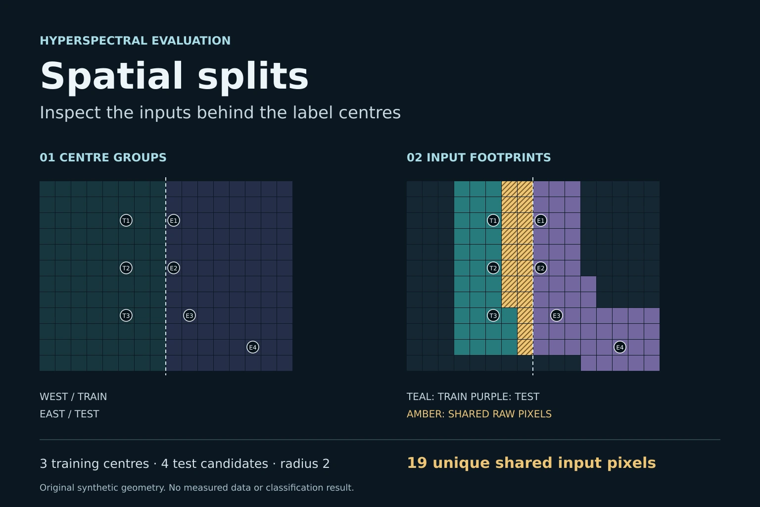
Use a 12 × 16 grid with zero-based (row,column) coordinates. The three training centres are (2,5), (5,5) and (8,5). The four candidate test centres are (2,8), (5,8), (8,9) and (10,13). All training centres lie in the west region, columns 0–7. All test centres lie in the east region, columns 8–15.
With radius 2, each interior patch is 5 × 5. The training-input union contains 55 unique pixels; the candidate test-input union contains 74. Their intersection contains 19 unique raw pixels. Seven train/test patch pairs overlap, and three of the four test candidates share input with training. All label centres and centre-group IDs remain separated.
The candidate-wise shared counts are 10, 10, 5 and 0. Adding them gives 25 because some shared pixels occur in more than one test patch. The union intersection is the correct answer to “How many distinct raw pixels are shared?” Keep this quantity separate from the number of overlapping examples or pairs.
The last test patch contains 20 pixels because it is clipped at the lower edge. A real pipeline may instead discard edge centres or pad its inputs. That choice changes the support audit and must be recorded. The inspector below clips patches and does not simulate padding.
SYNTHETIC GEOMETRY LAB · NO MODEL TRAINING
Audit the inputs behind a split
A 12 × 16 grid, several training and test centres, and exact square-patch intersections. Choose a preset, then change the radius or coordinates.
T: training centre · E: candidate evaluation centre · ×: excluded candidate
Teal: train input · purple: test input · amber hatch: shared input
| Centre | Class / group | Shared pixels | Decision |
|---|
| Synthetic class | Train | Candidate test | Retained test | Excluded |
|---|
Scope: every number is calculated from this synthetic grid. Zero overlap checks direct input sharing only. It cannot establish statistical independence, preprocessing isolation or generalisation to another scene. The manifest contains settings, candidate decisions, class counts and centre/input masks. It contains no accuracy score.
Use the full support, then test its intersection
For a square patch of radius r around a centre, include every grid coordinate within r rows and r columns. Two equal-radius patches on this rectangular grid intersect exactly when the Chebyshev distance between their centres is at most 2r. Chebyshev distance is the larger of the absolute row and column differences.
The threshold includes equality. At a centre distance of 2r, the patches can still share an edge row, edge column or corner pixel. With r = 2, centres (2,5) and (2,9) share a column of five pixels; (2,5) and (2,10) share none. A rule that rejects distances strictly smaller than 2r misses the touching case.
For several examples, form the union of all training footprints and the union of all evaluation footprints, then intersect those two sets. The supplied JavaScript enumerates actual coordinates, so it also handles clipped edges. Its tests compare this enumeration with the distance rule across every pair of centres on the synthetic grid.
Use a different support calculation when the pipeline reads different context. A local filter applied before patch extraction can expand raw input support. Graph neighbours can cross a spatial boundary. Whole-image attention can connect distant locations. A patch-radius slider cannot certify those pipelines; trace the observations that can influence each prediction.
Group splitting keeps identifiers apart; geometry still needs checking
The official GroupKFold documentation specifies non-overlapping groups across train and test, with each group appearing in a test fold once. The number of distinct groups must support the chosen number of folds. The caller supplies those group identifiers.
Choose identifiers that represent the held-out unit: scene, acquisition, field or another defensible sampling unit. Assigning every pixel its own group supplies no meaningful scene separation. Assigning centre pixels to neighbouring tiles can prevent shared tile IDs while their patches cross the tile boundary, exactly as in the worked example.
Inspect centre-group intersection and raw-input intersection after each split. When the evaluation requires unseen groups and disjoint inputs, apply both conditions. The inspector’s third preset shows the reverse case: distant patches can have zero shared input while their centres still belong to the same west-region group. Neither check substitutes for the other.
Freeze the outer held-out groups, then perform model selection inside the remaining development data with a validation design that respects the intended separation. Repeatedly choosing settings from the final test score changes its role. Save the selected indices so every model comparison uses the same examples.
Exclusion changes the test population
Enable overlap exclusion in the worked example. Three test candidates are removed; only (10,13) remains. The retained test input has zero intersection with training input, but 75% of the candidate centres have been discarded. That change belongs in the result, alongside any later performance metric.
The toy class map places A in rows 0–3, B in rows 4–7 and C in rows 8–11. Training contains one centre from each class. Before exclusion, evaluation contains A: 1, B: 1 and C: 2. Afterwards it contains A: 0, B: 0 and C: 1. No score computed on the retained set could describe test performance for A or B.
On a real map, inspect the excluded locations and their class counts. Boundary regions, small objects or rare classes may be removed unevenly. Report both the candidate pool and the retained evaluation population. If a class has no test support, mark its class-wise result as unavailable and state how any average treats it.
If separation leaves too little support for the intended claim, revise the data collection or split design before testing models. Do not quietly reduce the buffer after seeing which choice produces a favourable score. A larger exclusion zone is a design choice with a coverage cost, rather than an automatic improvement in every evaluation.
Declare target-feature access and preprocessing
For an inductive held-out evaluation, learn fitted transformations from the training partition, then apply the fixed transformation to held-out examples. This includes quantities such as standardisation statistics, PCA components and selected features. The scikit-learn data-leakage guidance documents this boundary and explains how pipelines keep fitting inside the appropriate cross-validation partition.
An experiment can deliberately allow unlabelled target observations during fitting. Declare that transductive access: which target spectra or spatial structure are visible, at which stage, and whether the model is adapted to those observations. For example, constructing a graph jointly over training and target features exposes target structure even if the target labels are hidden. The official label-propagation documentation describes building a graph over all supplied observations.
Keep target labels reserved for evaluation under that protocol. State any exceptions, such as a separately allocated target-domain validation label budget, rather than calling the whole target set unseen. A transductive result answers a different access condition from deployment where new observations arrive after training.
A coordinate audit cannot inspect fitted statistics, external pretraining data or model-selection history. Record those in the experiment manifest alongside the masks. Direct geometric separation is one verified property of the experiment, not a verdict that every possible leakage path has been closed.
Save the split as an inspectable artefact
A seed alone does not identify the evaluation set. Changes to pixel ordering, the valid-data mask, the label map or the sampling implementation can produce different indices. Preserve the actual selected centres and the information needed to interpret them.
The inspector exports a JSON manifest and a row-per-pixel CSV. Both are computed from the current setup. The JSON stores patch geometry, border handling, group rules, candidate decisions, class counts and binary masks. The CSV separates centre membership from input-footprint membership, making the two boundaries visible in ordinary analysis tools.
An excluded-centre mask means that a coordinate is not scored as a retained test target. It does not mean that its spectrum is absent from every retained patch. If a protocol forbids access to an entire region, audit the full input support against that region mask as an additional constraint.
For real experiments, extend this teaching manifest with dataset and annotation versions, source-file checksums, scene or acquisition identifiers, georeferencing and ground sampling distance, valid-data rules, validation masks, software versions and the declared preprocessing fit scope. Keep sensitive or non-public dataset details in the appropriate private record.
- Archive train, validation, candidate test, retained test and excluded-centre indices, with the coordinate convention.
- Save group membership, patch or receptive-field support, border policy and the exact exclusion rule.
- Report sample and class counts before and after filtering, plus shared raw-input counts.
- Record all uses of unlabelled target features, test labels, pretrained weights and tuning data.
- Version the split-generation code and run its overlap assertions before fitting each model.
Report the property you checked and the claim it supports
A useful methods paragraph names the prediction setting first, then the reserved unit, permitted data access, input support, exclusion rule and remaining class coverage. “Spatial split” on its own leaves all of those choices open.
For this worked example, an accurate report is: “On a synthetic 12 × 16 grid, training and candidate test centres occupied separate west/east regions. Radius-2 square patches were clipped at image edges. The candidate split shared 19 unique raw input pixels. Removing directly overlapping test patches retained one of four candidates and eliminated direct input sharing; only synthetic class C remained represented in evaluation.”
That paragraph reports an exact geometry calculation. It contains no classification result. For a real experiment, follow it with performance measured on the named population, uncertainty appropriate to the sampling units, and the limits of transfer supported by the available scenes or acquisitions. A buffered within-scene result still requires separate evidence before it becomes a cross-scene claim.
Frequently asked questions
Is a random pixel split always wrong?
Its interpretation depends on the prediction task and permitted information. Describe a same-scene interpolation setting explicitly, including patch overlap and any access to unlabelled target features. It does not establish transfer to a new scene.
Does GroupKFold prevent patch overlap?
It separates the group identifiers supplied for examples. If neighbouring groups share raw patch inputs, those inputs can still overlap. Audit the actual support after splitting.
How large should the buffer be?
For equal square patches of radius r, rejecting test centres at Chebyshev distance at most 2r from training centres removes direct patch sharing. Other input supports need their own calculation. A further separation margin requires a task-specific justification.
Why is the total shared-pixel count smaller than the sum per test patch?
Several test patches can contain the same raw pixel. The union-intersection count includes that pixel once; summing candidate-level counts can include it several times.
Can zero overlap be called leakage-free?
Zero overlap establishes only the checked geometric property. Inspect preprocessing, label access, graph construction, tuning and pretraining separately, and do not infer statistical independence or cross-scene transfer.
Does this lab use real HSI data or report model performance?
No. It enumerates square patches on a synthetic grid and exports their exact masks and counts. There are no measured spectra, fitted models or accuracy estimates.
References and further reading
- Liang et al. (2016). On the Sampling Strategy for Evaluation of Spectral-spatial Methods in Hyperspectral Image Classification
- scikit-learn. GroupKFold API documentation
- scikit-learn. Common pitfalls: data leakage and preprocessing
- scikit-learn. Semi-supervised learning: label propagation
- scikit-learn. Cross-validation iterators for grouped data
Reader feedback
Reads since 1 October 2026: at least 15 seconds with the article visible, counted once per browser per day. Reactions are anonymous and can be changed.
Loading reader feedback…
Discuss this article
Ask a technical question, challenge an assumption or share evidence from your own work.