
When one label throws away part of the answer
A hyperspectral pixel records a spectrum over a finite spatial footprint. That footprint can contain several surface components, and the light reaching the sensor can also involve interactions between them. A single class label compresses this measurement into one decision. Whether that compression is useful depends on the question.
If the task asks which land-cover class best describes a location, classification may be appropriate. If it asks how much each candidate component contributes under a mixing model, an abundance estimate is closer to the desired output. A minority component can matter even when it would never win a dominant-class decision. The small-object smoothing guide considers a related loss of detail across neighbouring pixels; here the ambiguity is within a spectrum.
Rasti and colleagues’ HySUPP paper organises linear unmixing into known-endmember, library-based and blind settings, and provides an open-source package for reproducible comparisons. This guide takes a narrower route: a transparent, two- or three-component example whose generating coefficients are known. It explains what a successful reconstruction can establish and where that evidence stops. [1]
Separate a class probability from a mixing coefficient
A classifier’s probability concerns the assigned class under its labelling scheme and model. An estimate such as P(class A | spectrum) = 0.8 does not say that 80% of the pixel’s area contains A. A pure pixel can receive uncertain class probabilities because two classes look similar; a mixed pixel can receive a confident dominant-class label.
Probability calibration asks whether stated confidence agrees with empirical correctness frequency under an evaluation protocol. Guo and colleagues study that issue for neural classifiers. Calibration would improve the interpretation of a class-probability estimate, but would not turn it into a material fraction. Training against measured fractional targets would define a different prediction problem. [2]
Likewise, a coefficient that sums with others to one is not automatically a physical proportion. Under an appropriate areal linear-mixture model, with compatible illumination and measurement conditions, an abundance may represent a footprint fraction. Intimately mixed grains, multiple scattering, coatings and changing optical properties require additional modelling. In particular, these coefficients do not establish a flour sample’s mass composition.
| Output | Question answered | Evidence still needed |
|---|---|---|
| Class probability | How likely is this class decision under the model? | Calibration and appropriate class labels |
| Estimated abundance | Which coefficients best fit the chosen mixing model? | Endmember validity, identifiability and fractional reference data |
| Reconstruction residual | What signal is left unexplained by this fit? | Diagnosis of discrepancy and validation of material identity |
Build the smallest model you can inspect
Write the linear model as y = Ea + ε. The vector y contains the observed bands; the columns of E are candidate endmember spectra; a contains their coefficients; and ε collects noise and model discrepancy. The usual fully constrained least-squares problem minimises the squared reconstruction residual while imposing aₖ ≥ 0 and Σaₖ = 1. Heinz and Chang’s paper develops fully constrained linear spectral mixture analysis. [3]
For two endmembers, the feasible spectra form the line segment joining the two curves in spectral space. Three affinely independent endmembers form a triangle. The constraints restrict the fit to this convex hull. They prevent negative fractions and enforce closure, but they cannot add a missing component or validate the selected endmembers.
The lab below uses 81 equally weighted bands from 450 to 1250 nm. Its A, B and C curves are original analytic functions with arbitrary shapes and no physical material identities. The default observation is exactly 0.4A + 0.3B + 0.3C. The browser evaluates all vertices and edges, plus a feasible triangle-interior solution, rather than relying on a training process or an iterative optimiser.
Interactive synthetic experiment · runs in your browser
One spectrum, several possible explanations
Set the generating fractions, then fit a nonnegative, sum-to-one linear mixture. A, B and C are anonymous analytic curves, not measured materials. No trained classifier or research benchmark is running.
The default generating fractions are A 40%, B 30%, C 30%. They always sum to 100%.
With correct, distinct endmembers and no perturbation, this constructed mixture can be recovered to floating-point precision.
● Observed – – Fitted A · B · C: generating endmembers
Residual = observed − fitted, in dimensionless signal units. The labelled vertical scale adapts to the residual.
| Component | Generating fraction | Estimated fraction | Difference |
|---|---|---|---|
| A | 40.00% | 40.00% | 0.00 pp |
| B | 30.00% | 30.00% | 0.00 pp |
| C | 30.00% | 30.00% | 0.00 pp |
Known-endmember coefficient recovery is different from discovering unknown endmembers from an image.
Stress the assumptions
These deterministic perturbations are sensitivity probes, not a sensor-noise distribution or confidence interval. Along B − A, a small spectral change can be absorbed as a change in fractions. When A = B that contrast is zero, so this probe adds no perturbation.
The default example is shown above. Controls become available when the interactive module loads.
Interpretation limit: estimated fractions belong to the selected model and dictionary. A small residual does not prove the correct materials were used. These coefficients are neither class probabilities nor a sample’s mass composition.
Equations, data and numerical scope
The linear signal is y = Σ aₖeₖ, where aₖ ≥ 0 and Σ aₖ = 1. The fit minimises Σᵦ(yᵦ − Σₖaₖeₖᵦ)². The solver checks all vertices, edges and the feasible triangle interior for at most three endmembers. Degenerate interiors are covered by their edges; one representative minimiser is shown.
The nonlinear preset adds γΣᵢ<ⱼaᵢaⱼ(eᵢ ⊙ eⱼ), an explicit toy bilinear term. It does not simulate an instrument, flour chemistry or a full radiative-transfer model. There is no clipping, normalisation or learned preprocessing.
The grid is 450–1250 nm every 10 nm, with 81 equally weighted bands. Spectral RMSE averages squared residuals across bands; coefficient RMSE averages squared fraction errors across generating components, counting an excluded component as zero. “pp” means percentage points. Downloads contain the equations’ inputs and original synthetic output.
Read the HySUPP overview and package paper for broader methods and reproducible research comparisons. This small browser solver is independently authored and is not HySUPP.
Start with recovery, then deliberately remove information
Choose “Correct endmembers”. With no perturbation, the estimated fractions match the generating fractions to floating-point precision. Try the two-component mode and a pure endpoint. The sum remains one because B receives the amount left after A; with three components, its control allocates a share of that remainder and C receives the rest.
This is a numerical recovery test under a model that is true by construction. It verifies the implementation and illustrates the constraints. It does not demonstrate a method’s accuracy on measured imagery. There is no classifier, GPU workload or published benchmark running behind the controls.
Now choose “Very similar A and B”. Here B becomes 0.96A + 0.04B₀, where B₀ is the original B curve. The preset adds a deterministic perturbation with only 0.001 RMS, directed along B − A. The default A estimate changes from about 16.52% to 63.48% when that perturbation is flipped. Both fits have residuals near numerical zero. The approximately 46.96 percentage-point swing shows that small spectral differences can support large coefficient differences.
This deliberately aligned perturbation is a stress test, not a random noise model, expected error rate or confidence interval. A real uncertainty analysis needs an observation-error model and a treatment of endmember uncertainty. The alternate band-wise ripple lets you compare a different perturbation direction.
A small residual can hide a missing material
In “C missing from the fit”, all three distinct curves generate the observation, but only A and B are available to the solver. It allocates the entire coefficient sum to them. At the default 40/30/30 mixture, spectral RMSE is about 0.03772. The structured residual is useful evidence that the selected linear model is inadequate for this observation.
That evidence does not uniquely diagnose the cause. A missing component, spectral mismatch, nonlinear interaction, calibration error or inappropriate band weighting can all contribute. Inspect the residual against wavelength, rather than retaining only one aggregate score.
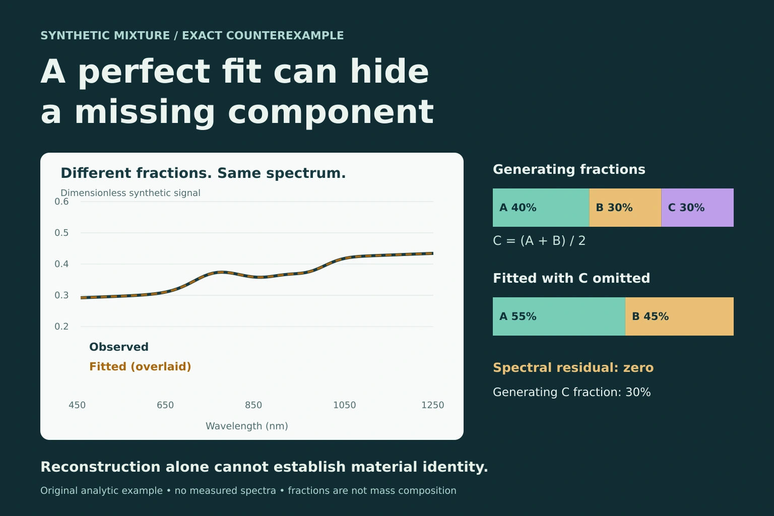
The next preset is the stronger counterexample. In “Missing C hidden by A + B”, the generating C curve is exactly (A + B)/2. The observation 0.4A + 0.3B + 0.3C can therefore be written as 0.55A + 0.45B. The fitter excludes C, yet reconstructs the signal exactly. The known generating coefficient of C is 30%; the model has no slot in which to report it.
This algebraic example establishes a specific limitation: reconstruction fidelity alone cannot prove correct material identity or composition. It also explains why reporting both spectral error and abundance error is useful when valid abundance reference data exist. In the lab, coefficient RMSE counts an excluded component as zero and averages errors over every generating component.
Distinguish non-uniqueness from numerical instability
“Identical A and B” makes the issue exact. With A = B, the default observation is 0.7A + 0.3C. Splits of 70/0/30, 0/70/30 and 40/30/30 all produce the same spectrum. Only the combined A-plus-B coefficient is determined. The solver returns a reproducible representative solution and explicitly displays an alternative; its preference is not evidence about the generating split.
Near-identical endmembers create a related but different problem. A fixed, affinely independent dictionary can still give a unique least-squares solution, while that solution is highly sensitive to small measurement or endmember changes. Exact uniqueness and practical stability should be assessed separately. A large number of bands does not guarantee informative differences between the candidate curves.
Blind unmixing must also infer the endmembers. Lin and colleagues analyse identifiability of a minimum-volume enclosing simplex in the noiseless, no-pure-pixel case. Their guarantees depend on conditions on how the abundance vectors populate the simplex. The result does not say that arbitrary mixtures reveal unique endmembers, or that a small reconstruction error verifies the required conditions. [4]
The browser experiment estimates coefficients for a supplied dictionary. It neither extracts endmembers from an image nor demonstrates a blind-identification theorem. Pure pixels can help some methods, but their presence, absence or apparent purity must be evaluated under the particular method and acquisition model.
Treat the endmember library as a scientific choice
A reference spectrum needs a compatible measurement domain: wavelength support, spectral response, units, calibration and relevant physical conditions. Laboratory measurements and image pixels are not interchangeable merely because both have a wavelength axis. Material variability can require several spectra or an explicit variability model; Halimi and colleagues give a probabilistic unmixing treatment of changing endmembers. [5]
The USGS Spectral Library Version 7 is a primary resource with spectra measured in laboratory, field and airborne settings, together with sample and measurement documentation. For a real experiment, select and cite the exact records and inspect their metadata. Resample using a justified sensor-response model where necessary, and check the record’s reuse terms. [6]
No USGS samples or figures are embedded here. Keeping the curves analytic makes the counterexamples exact and avoids implying that arbitrary synthetic mixing reproduces the behaviour of a named mineral, crop or powder. The downloadable JSON contains the actual endmembers, generating fractions, fitted fractions and residuals used by the current display.
Check the linear assumption before interpreting fractions
The nonlinear preset adds γΣᵢ<ⱼaᵢaⱼ(eᵢ ⊙ eⱼ), where ⊙ means multiplication band by band. This is an explicit toy bilinear interaction. The fitting model remains linear, so its coefficients can move to absorb some of the additional signal. Setting the interaction strength to zero returns to the linear generating model.
Halimi, Altmann, Dobigeon and Tourneret’s primary study develops a generalised bilinear model and an estimation method for nonlinear hyperspectral unmixing. Its scientific role here is to show that interactions require model choices beyond the linear sum. This lab does not reproduce that paper’s algorithm, experiments or physical validation. [7]
Unconstrained least squares followed by clipping negative coefficients and renormalising is not generally the constrained least-squares solution. If sum-to-one is inappropriate because of illumination or an omitted contribution, enforcing it can redistribute the mismatch into misleading fractions. Decide the physical representation and constraints first, then test the resulting model; do not interpret constraint satisfaction as proof that the assumptions hold.
Report what was recovered and what remains unresolved
A useful unmixing report identifies the input quantity and units, sensor bands and masks, endmember provenance, number of components, mixing model, constraints, optimiser and tolerances. State whether the task used known signatures, a candidate library or endmembers estimated from the data. Record how preprocessing and parameter selection were separated from evaluation.
Report the residual spectrum and an aggregate spectral error, then add reference-based coefficient errors when appropriate ground truth exists. If estimated endmembers can be permuted, make the matching protocol explicit before comparing coefficients. Examine sensitivity to plausible endmember changes, missing components, band selection and observation errors. A smooth abundance map can still be wrong, just as a smooth classification map can erase a small object.
For a classification application, decide how any abundance estimates contribute to the final decision and evaluate that decision separately. Hard-label overall accuracy cannot validate fractional recovery. Conversely, low abundance error in a synthetic mixture does not establish cross-scene classification quality. The metric workbench and spatial-split guide cover those distinct evaluation questions.
The practical stopping point is a claim with a clear scope: these coefficients explain this observation under this dictionary and mixing model, with these validation and sensitivity results. Stronger statements about material identity, area or chemistry need evidence appropriate to those quantities.
Frequently asked questions
Does 80% class confidence mean 80% abundance?
No. Class probability concerns a class decision under a model and labelling scheme. Abundance is a coefficient in a mixing model. Calibration does not make the two quantities equivalent.
Does zero reconstruction error prove the right materials were identified?
No. The hidden-C example has an exact two-curve reconstruction while omitting a component used to generate the observation. Non-unique dictionaries can support several equally good explanations.
Is this lab using real USGS spectra?
No. All curves are original analytic synthetic endmembers. USGS is linked as a documented primary resource for real measurements, but none of its spectra or figures is embedded.
Can the fractions be read as chemical mass percentages?
No. The lab reports coefficients of a synthetic signal model. Mass composition requires an appropriate calibrated physical or empirical relationship and independent validation.
Why can a tiny spectral perturbation cause a large coefficient change?
When candidate endmembers are very similar, reallocating signal between them changes the reconstructed spectrum only slightly. A unique fit can therefore be highly sensitive. Exact duplicate endmembers make the split non-unique.
Is the perturbation-flip result a confidence interval?
No. It compares two deterministic sensitivity probes with opposite signs. It does not define a probability distribution, coverage level or real sensor uncertainty.
References and further reading
- Rasti, B., Zouaoui, A., Mairal, J. & Chanussot, J. (2024). Image Processing and Machine Learning for Hyperspectral Unmixing: An Overview and the HySUPP Python Package. IEEE TGRS. DOI: 10.1109/TGRS.2024.3393570.
- Guo, C., Pleiss, G., Sun, Y. & Weinberger, K. Q. (2017). On Calibration of Modern Neural Networks. ICML, PMLR 70, 1321–1330.
- Heinz, D. C. & Chang, C.-I. (2001). Fully Constrained Least Squares Linear Spectral Mixture Analysis Method for Material Quantification in Hyperspectral Imagery. IEEE TGRS 39(3), 529–545.
- Lin, C.-H., Ma, W.-K., Li, W.-C., Chi, C.-Y. & Ambikapathi, A. (2015). Identifiability of the Simplex Volume Minimization Criterion for Blind Hyperspectral Unmixing: The No-Pure-Pixel Case. IEEE TGRS 53(10), 5530–5546. DOI: 10.1109/TGRS.2015.2424719.
- Halimi, A., Dobigeon, N. & Tourneret, J.-Y. Unsupervised Unmixing of Hyperspectral Images Accounting for Endmember Variability. Primary research preprint, arXiv:1406.5071.
- Kokaly, R. F. et al. (2017). USGS Spectral Library Version 7. U.S. Geological Survey Data Series 1035, 61 pp. DOI: 10.3133/ds1035.
- Halimi, A., Altmann, Y., Dobigeon, N. & Tourneret, J.-Y. (2011). Nonlinear Unmixing of Hyperspectral Images Using a Generalized Bilinear Model. IEEE TGRS 49(11), 4153–4162. DOI: 10.1109/TGRS.2010.2098414.
Reader feedback
Reads since 1 October 2026: at least 15 seconds with the article visible, counted once per browser per day. Reactions are anonymous and can be changed.
Loading reader feedback…
Discuss this article
Ask a technical question, challenge an assumption or share evidence from your own work.