Train/Test Split: It’s Complicated. They Share a 27×27 Patch

Congratulations on discovering next door

Welcome to the lab. The model has a spectral branch, a spatial branch, an attention branch and, apparently, a family tree connecting the training set to the test set.

We have carefully shuffled the labelled pixels. We have fixed the seed. We have checked that no centre-pixel index occurs in both sets. Excellent. The train and test IDs are now legally separated.

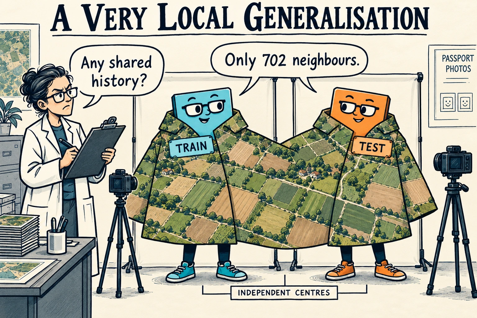
Their 27×27 patches are still living together.

Take two interior square patches whose centres are one column apart. Each contains 729 pixel locations. Their intersection contains 26×27 = 702 locations, or 96.3% of either patch. That number is geometry, not a reported accuracy. It assumes full, unpadded, axis-aligned patches of equal size. At image boundaries, or with different extraction rules, do the actual calculation.

We gave the samples different names and hoped the farmland would respect administrative boundaries.

This concern has a literature, which is inconvenient for anyone hoping to dismiss it as Reviewer 2 discovering subtraction. Liang and colleagues explicitly illustrated overlapping neighbourhoods in spectral-spatial HSI evaluation [1]. Nalepa and colleagues showed why held-out centre pixels can still appear inside training inputs [2]. The index assertion passes. The information-boundary question remains open.

Please specify which sort of leakage is attending

Before anyone declares an entire field fraudulent, put down the pitchfork. It has a spatial receptive field.

Patch overlap means two examples use some of the same raw pixel locations. A held-out pixel’s spectrum might occur inside a training patch while its class label remains hidden. This matters for the claim being tested, but it is not automatically test-label leakage.

Test-label leakage means held-out labels influence fitting or selection. Perhaps they enter a feature, a supervised preprocessing step, an early-stopping decision, or the increasingly spiritual process of choosing the architecture that looks best on the test table. Renaming that table “validation” after the camera-ready deadline does not repair the estimate.

Spatial autocorrelation means nearby observations are related. Even disjoint patches may belong to the same field, roof, soil regime or acquisition context. Geiß and colleagues distinguish intrinsic spatial dependence from the extra dependence introduced by spatial features [3]. Removing shared pixels does not make the landscape independent and identically distributed out of politeness.

Transductive access means the protocol permits information from the unlabeled target set during learning or adaptation. If the task is mapping a known scene with limited annotations, access to that scene can be entirely sensible. State exactly what was visible, including spectra, graph edges, preprocessing statistics and labels. A purely supervised local patch model is not automatically transductive just because neighbouring inputs overlap. The allowed information boundary decides the question.

Inductive evaluation tests a learned predictor on new examples under a protocol that keeps the evaluation set out of fitting and selection. For a claim about new scenes, a familiar scene with fresh pixel IDs is a weak substitute. The scene has not travelled anywhere. It has changed its name badge.

These distinctions are useful because “leakage” is otherwise a conference buffet: everyone points at something different and announces that the whole room is contaminated.

What exactly was meant to generalise

There are legitimate reasons to estimate performance on additional pixels in a partly labelled scene. A random labelled-pixel split may fit that deployment question, provided the label-sampling scheme and permitted scene access are explicit. It is not a certificate of fraud, nor a free pass to claim transfer to a new city, season or sensor.

If the question is performance on geographically separated regions, hold out regions. If it is new scenes, hold out whole scenes. If it is future acquisitions, respect time. If it is another sensor, test that shift rather than hoping a different random seed qualifies as hardware diversity.

Roberts and colleagues make the general principle explicit: the blocking strategy should follow the prediction objective and the dependence structure [4]. Applying that principle to HSI, interpolation across a known image and transfer to an unseen image are different estimands. The estimand is the thing you meant the number to estimate, before the number became emotionally important.

A lower spatially held-out score is not a forensic measurement of “percentage points caused by cheating”. Changing a split can change training diversity, class coverage, distance to training examples and the difficulty of prediction. Nalepa and colleagues discuss those complications in their own patch-based experiments [2]. A clean criticism must keep them visible.

“Spatial split is harder” can be true. Whether that difficulty is appropriate depends on where the model is going to work. A driving test becomes harder when the examiner asks you to leave the driveway. This is only unfair if the product is a driveway vehicle.

A small experiment with unusually honest ambitions

Open the interactive lab below. It generates an 80×56 synthetic scalar field, optionally smooths it, and assigns classes using a fixed zero threshold. No benchmark imagery, hyperspectral cube or published accuracy is involved.

The learner is deliberately embarrassing: coordinate-only one-nearest-neighbour classification. A test pixel inherits the label of its nearest training centre. It sees training labels and coordinates. It sees no spectra and no test labels. Liang and colleagues also examined coordinate-only classifiers to expose spatial structure in within-image evaluation [1]; our tiny implementation is an illustration, not a reproduction of their experiment.

Start with random centres, a 1×1 patch, no buffer and a smooth field. If the classifier does well, exact patch overlap cannot explain it: a single-pixel train input and a different single-pixel test input do not overlap. Spatial structure can still make nearby labels predictable. Now reduce smoothing. The field changes, and the usefulness of proximity changes with it.

Next enlarge the patch while keeping the field fixed and watch the overlap measure. Larger patches create more opportunity for shared inputs, although this toy also changes eligible centres and rebuilds the split. This coordinate-only learner never consumes patches. Do not credit a score change to patch information it never received. Patch size also changes the set of eligible interior centres, because this demonstration refuses to conceal padding behind the sofa.

Switch between random and blocked centres at the same settings. The training budget is matched exactly before buffering. The blocked mode fills a left-hand strip, with at most one partially filled edge column. It is one illustrative partition, not an optimal spatial cross-validation design. Its test geography and class balance can differ from the random split. Equal sample counts are a useful control; they are not a magical fairness amulet.

Finally press “Separate patch supports”. For patch width p, this excludes test centres within Chebyshev distance p−1 of any training centre. Two equal square patches overlap exactly when both centre-coordinate separations are at most p−1. The button therefore removes all shared input locations under this toy’s extraction rules. For scattered training centres and large patches, it may remove every test example. The display then says there is no test set. It does not helpfully manufacture zero accuracy.

Notice what survived the demonstration: explicit assumptions, a known label rule, visible exclusions and denominators. Notice what did not appear: a graph claiming that our new architecture beat the literature by a number selected for comic timing.

A buffer is not holy water

For two equal patches of radius r, excluding centre distances up to 2r in the Chebyshev metric prevents their supports from intersecting. For 27×27 patches, r is 13, so exclude distances of 26 or less. Excluding only 13 pixels protects one centre from entering the other patch; it does not necessarily separate both full patches.

Then inspect the rest of the pipeline. Smoothing, morphological profiles, superpixels, resampling and graph construction can create a larger information footprint than the patch shown in the methods figure. Global attention may make a tidy local buffer insufficient. Choose the boundary for the actual computation, not for the prettiest square in the diagram.

Geometric separation also leaves longer-range spatial correlation. A buffer width should be justified by the application, preprocessing support and relevant dependence scale, with sensitivity checks where feasible. There is no universally sanctified number of pixels that converts one farm into independent farms [3,4].

The evaluation protocol that survives its own appendix

Here is a practical repair, before the abstract develops another attention mechanism.

1. Write the deployment claim first. Name the target geography, acquisition setting and permitted unlabeled target access. Specify what the reported score estimates. Keep same-scene interpolation and new-scene transfer in separate results when both matter.
2. Split the appropriate units before fitting data-dependent steps. For an inductive protocol, fit normalisation, PCA, feature selection and other learned transformations using training data only, then apply them to validation and test data. Inside cross-validation, refit inside each training fold. For a transductive protocol, declare and evaluate target-data use explicitly instead of quietly borrowing it.
3. Audit support, class coverage and discarded data. Check centre-ID overlap and actual input-support overlap separately. Publish split masks, extraction rules, buffer distances, per-class counts and retained test counts. If a held-out scene contains a class absent from training, report the consequence and define whether that belongs to the intended task. Do not quietly solve it by reaching into the test labels.
4. Keep selection inside the boundary. Tune preprocessing, patch size, architecture and stopping on training/validation data. When resampling estimates the entire model-selection procedure, perform selection within the outer training folds, using inner splits that also respect the intended structure. Cawley and Talbot show how model-selection overfitting contaminates performance evaluation [5]. Nested selection addresses that problem; it does not independently fix spatial dependence.
5. Compare methods under the same rules. Match split masks, available labels, allowed imagery, preprocessing permissions and selection budgets. Report useful simple baselines, including spectral-only or coordinate-only diagnostics where appropriate. If a spectral-spatial method gains from neighbourhood information, that is interesting. Specify the deployment setting in which that gain is available.
6. Put the right experiment inside the error bars. Multiple optimiser seeds on one scene describe some training variability conditional on that scene and split. They are not multiple independently sampled scenes. Report which sources varied, preserve paired comparisons, and base geographic generalisation uncertainty on appropriate scene or region units when enough such units exist. With very few independent scenes, say the evidence is limited instead of promoting pixels to international correspondents [4,6].

Bouthillier and colleagues distinguish several sources of benchmark variance, including data sampling and initialisation [6]. A small seed-only standard deviation can be real and precisely answer a much smaller question than the abstract suggests.

Five runs of the same farm are still one farm. The maize has not attended five universities.

The punchline should survive replication

The problem is not that spatial context works. Spatial context is often the point. The problem is asking a local interpolation experiment to perform overseas duties without the paperwork.

Keep the strong result when its protocol supports the claim. Narrow the claim when that is what the evidence permits. Run a genuinely separated evaluation when the application needs one. Release enough of the splitting and selection procedure that another researcher can discover whether the result survives a change of neighbourhood.

And when someone asks whether the training and test sets are independent, perhaps begin with something more informative than:

“We used different colours.”

References and further reading

1. Liang, J., Zhou, J., Qian, Y., Wen, L., Bai, X., and Gao, Y. (2017). “On the Sampling Strategy for Evaluation of Spectral-Spatial Methods in Hyperspectral Image Classification.” IEEE Transactions on Geoscience and Remote Sensing, 55(2), 862–880. DOI · Open manuscript. Relevant: §III, Table I; §IV, Fig. 6; §VI.
2. Nalepa, J., Myller, M., and Kawulok, M. (2019). “Validating Hyperspectral Image Segmentation.” IEEE Geoscience and Remote Sensing Letters, 16(8), 1264–1268. DOI · Open manuscript. Relevant: §I, Figs. 1–2; §§II–III; class-coverage and representativeness caveats.
3. Geiß, C., Aravena Pelizari, P., Schrade, H., Brenning, A., and Taubenböck, H. (2017). “On the Effect of Spatially Non-Disjoint Training and Test Samples on Estimated Model Generalization Capabilities in Supervised Classification With Spatial Features.” IEEE Geoscience and Remote Sensing Letters, 14(11), 2008–2012. DOI · DLR repository. Relevant: §II, Fig. 1; §IV, Fig. 3.
4. Roberts, D. R., et al. (2017). “Cross-validation strategies for data with temporal, spatial, hierarchical, or phylogenetic structure.” Ecography, 40(8), 913–929. Full text and DOI. Relevant: Table 1; “Guidance: how to block”, Steps 1–3. General structured-data guidance; HSI deployment examples here are the article’s application of it.
5. Cawley, G. C., and Talbot, N. L. C. (2010). “On Over-fitting in Model Selection and Subsequent Selection Bias in Performance Evaluation.” Journal of Machine Learning Research, 11(70), 2079–2107. Official paper. Relevant: §§5.1–5.3. Addresses selection bias, not spatial overlap itself.
6. Bouthillier, X., et al. (2021). “Accounting for Variance in Machine Learning Benchmarks.” Proceedings of Machine Learning and Systems, 3. Official paper. Relevant: §2.2, Fig. 1; §3.2. General ML variance study, not an HSI benchmark.

Editorial note: the characters and dialogue are fictional. The target of the satire is methodological overclaiming. Cited authors supply evidence and useful qualifications; they are not presented as the fictional researchers. The interactive results are computed synthetic examples, not claims about published models.