
Learn a useful representation, then prove what transfers
Self-supervised learning uses structure in the observations to create a training signal without the downstream human labels. In hyperspectral imaging, an encoder might learn to agree across two views of a patch, predict hidden wavelengths, or reconstruct missing spatial regions. The useful outcome is a representation that helps an independently evaluated task. A falling pretraining loss, by itself, does not establish that outcome.
The hard decisions usually precede the architecture: which acquisitions may enter pretraining, what transformations preserve the information the task needs, what a masked token represents, and which locations remain genuinely unseen. A model can learn scene identity, sensor artifacts or interpolation shortcuts while looking successful on the pretext task. This guide turns those possibilities into explicit checks.
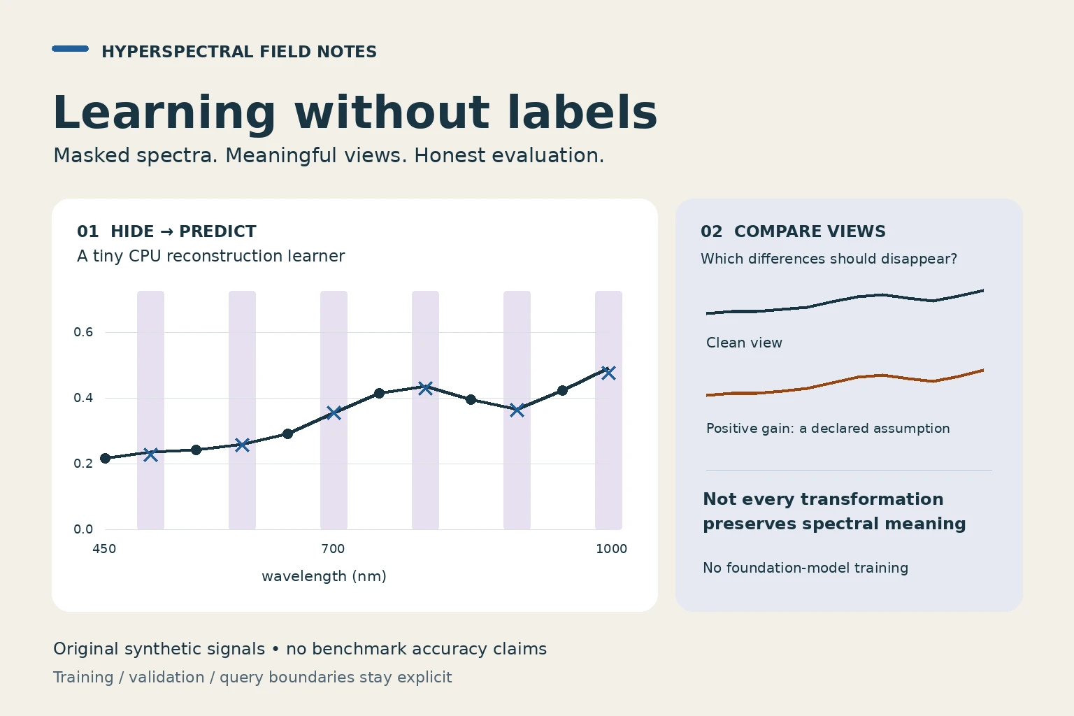
The companion lab fits a tiny masked linear reconstruction model on 72 original synthetic spectra, evaluates reconstruction on 24 separate validation spectra, and lets you inspect 24 additional queries. It also computes contrastive-loss arithmetic on raw spectral vectors. No foundation-model weights, measured image cubes or GPU training are used. The exercise is a reproducible mechanism demonstration, not an HSI benchmark or a pretrained foundation model.
Define the data contract before choosing an objective
Write down the physical quantity and processing level: radiance, reflectance, digital numbers or already standardized values. Preserve wavelength centres, wavelength units, channel order, band exclusions and validity masks alongside every tensor. Spatial sampling, acquisition date, atmospheric correction and scene identifiers are also part of the input contract. Two arrays with the same channel count need not describe comparable observations.
Fit data-dependent normalization, PCA, band selection and other learned transforms only on the data pool allowed by the evaluation protocol. A fixed transformation supplied with a released checkpoint is a different case: document and reuse that checkpoint contract, then disclose its pretraining provenance. Do not quietly recompute normalization using a downstream test scene while describing the result as strict unseen-scene transfer.
Missing channels are not zero reflectance. Use a validity representation and exclude invalid target values from reconstruction losses. An artificial pretraining mask asks the model to predict an available measurement; a sensor-invalid band has no trustworthy target. Keep these two masks separate. Report the number of valid target elements contributing to each loss, especially when scenes have unequal missingness.
| Setting | Training signal or trainable part | Main audit question |
|---|---|---|
| Contrastive pretraining | Agreement of positive views against negative examples | Does the positive rule preserve the target? |
| Masked pretraining | Prediction of hidden valid measurements | Can a preprocessing shortcut reveal the answer? |
| Frozen linear probe | Only a linear task head; encoder and buffers fixed | Are frozen features useful under this label budget? |
| Adapter tuning | Declared adapter and head; most backbone fixed | How much target-domain fitting is allowed? |
| Full fine-tuning | Encoder and task head updated | Is the comparison fair on data and selection effort? |
Contrastive learning: decide which differences should disappear
SimCLR builds positive pairs from two augmented views, maps them through an encoder and projection head, and contrasts the pair against other examples. Its study makes augmentation composition central to the learning problem. That is the transferable lesson here, not a claim that its RGB transformations are automatically valid for hyperspectral data. [1]
For one anchor i and its positive j, a normalized temperature-scaled loss is −log[exp(sim(z_i,z_j)/τ) / sum over k≠i exp(sim(z_i,z_k)/τ)]. The positive belongs in the denominator; the anchor itself does not. A full SimCLR-style minibatch loss averages directed positive-pair terms. The lab deliberately displays one anchor with one positive and three negatives, so its number is not a full training run. [1]
In an HSI experiment, the positive-pair rule is a scientific assumption. A crop that removes the target material may create a false positive pair. Two dates from one field can differ in crop, moisture or management. Treating them as identical may erase exactly what a change-detection or biochemical task needs. Choose invariance for the downstream target, not because a transformation is fashionable.
Negatives are assumptions too. Adjacent patches can share the same material while being treated as different instances; repeated acquisitions can be near duplicates. False negatives can make an instance-discrimination objective conflict with a material-classification goal. Record how batches are sampled across scenes, locations and dates. When interpreting losses, keep candidate count and temperature fixed: changing either changes the number even if the representations do not improve.
Sources: [1]
Interactive CPU lab · original synthetic spectra
Hide a spectrum. Inspect the learning signal.
A tiny ridge model really fits on 72 training curves. Separate validation and inspection queries reveal its errors. The second panel explains contrastive arithmetic without training an encoder. This is not a trained foundation model.
1. Predict the hidden wavelengths
● Visible input · × Ridge prediction · solid line: target for inspection · shaded bands: hidden
Hidden-band MSE: training 1.514e-4 · validation 1.367e-4 · inspection query 5.666e-5. Validation mean-only baseline: 6.941e-3. Lower is better for this reconstruction task only.
Errors use only hidden channels and have squared signal units. Each mask setting fits a separate model; a lower query score after exploration is not final-test evidence.
2. What should count as a positive view?
Solid line: clean query · dashed line: transformed view
Reversing values while keeping wavelength metadata fixed changes spectral meaning. This is an intentionally invalid positive view, not a recommended augmentation.
One-anchor contrastive loss: 1.339962. Positive share: 26.19%. These are loss terms, not task accuracy.
Bars are denominator softmax shares, not class probabilities or confidence. Raw unit-normalized spectra act as demo embeddings. Three negatives are fixed training curves. Positive gain leaves cosine similarity unchanged; no encoder learned this invariance. Jitter is a sine perturbation, not a calibrated sensor-noise model.
Inspect every wavelength and the numeric fixtures
| nm | Mask | Target | Ridge | Positive view |
|---|---|---|---|---|
| 450 | Visible | 0.216593 | 0.216593 | 0.216593 |
| 500 | Hidden | 0.235273 | 0.227440 | 0.235273 |
| 550 | Visible | 0.240897 | 0.240897 | 0.240897 |
| 600 | Hidden | 0.258998 | 0.256930 | 0.258998 |
| 650 | Visible | 0.291512 | 0.291512 | 0.291512 |
| 700 | Hidden | 0.354026 | 0.354540 | 0.354026 |
| 750 | Visible | 0.413605 | 0.413605 | 0.413605 |
| 800 | Hidden | 0.435280 | 0.429673 | 0.435280 |
| 850 | Visible | 0.394864 | 0.394864 | 0.394864 |
| 900 | Hidden | 0.365010 | 0.364311 | 0.365010 |
| 950 | Visible | 0.422350 | 0.422350 | 0.422350 |
| 1000 | Hidden | 0.491642 | 0.476081 | 0.491642 |
Known answers: hidden-band MSE fixture = 0.04; three equal candidate logits give ln(3) = 1.098612289; similarities [1, 0, −1] at τ = 1 give loss 0.407605964. Tests are in the source download.
Download runnable CPU source · Download all synthetic spectra
Static defaults shown. JavaScript enables controls; the Python code runs independently.
Masked prediction: decide what information must be inferred
The original MAE work uses an encoder on visible image patches and a lightweight decoder that reconstructs masked content. Its image experiments demonstrate a particular architecture and masking setup. They do not establish a universal masking ratio for every HSI sensor, tokenization or task. [2]
An HSI mask may hide individual channels, contiguous wavelength groups, spatial patches, or spectral-spatial blocks. These are different prediction problems. Scattered channels often retain nearby spectral clues. A contiguous interval can remove an entire feature. A spatial-only mask may preserve all wavelengths at neighbouring pixels. A joint mask can remove both kinds of context, but it can also become too ambiguous to be useful.
For an explicit masked squared-error objective, L = sum over masked-and-valid elements of (prediction − target)² divided by the count of those elements. A zero count is undefined and should be skipped or reported unavailable, not emitted as a perfect zero. The lab scores only its hidden channels. Its visible-channel values are passed through unchanged and never counted as successful reconstruction.
Prevent target leakage before tokenization. A convolution or smoothing transform that mixes a hidden band into a visible feature can give the answer away before masking begins. Masking a token after constructing it from the full unmasked cube is not necessarily the same as withholding the raw measurements. Trace receptive fields, pooling, normalization and skip connections. The correct order depends on the intended method, but the information available to the encoder must match the stated pretext task.
Reconstruction rewards predictable detail. A smooth-spectrum interpolator may achieve low error without learning a representation that separates rare classes. Strong high-variance bands can dominate unweighted MSE. Band-standardized targets, alternative losses or loss weights change the objective and need train-only fitting plus disclosure. Pair the pretext score with downstream evaluation and simple reconstruction baselines.
Sources: [2]
Augment spectra with a task-specific physical justification
A positive global gain can be a useful stress test for illumination or scale variation when the downstream target should ignore amplitude. It is not a complete model of illumination, reflectance anisotropy or atmospheric correction. If absolute reflectance carries the target signal, forcing gain invariance may remove useful information. In the lab, gain is explicitly a numerical transformation of a synthetic vector.
Small additive noise can test sensitivity, but a defensible augmentation should respect sensor noise structure and signal dependence when these are known. Independent equal-variance jitter on every band is only a teaching approximation. Clipping to a nominal interval changes the noise distribution near its boundaries. The lab uses a deterministic sine perturbation, reports its amplitude, and does not silently clip values.
Spatial flips or rotations can be reasonable for an orientation-insensitive label, provided masks and every aligned modality undergo the same transform. Random crops require retained target support; rescaling changes effective spatial resolution. Spectral dropout should carry an explicit missingness mask. A physically motivated sensor-response convolution may simulate a broader band, whereas arbitrary channel shuffling changes the relationship between wavelength and value.
Do not transplant RGB hue, saturation or channel permutations without a spectral interpretation. Wavelength jitter requires a supported resampling model and uncertainty assumptions; moving the axis labels is not calibration. The reverse-order control in the lab is intentionally an invalid positive-view example when wavelength metadata stay fixed. It demonstrates a failure to preserve meaning, rather than recommending a training augmentation.
For each transformation, save its range, probability, random seed, scientific rationale and the failure condition that would make it unsuitable. Compare a no-augmentation baseline and an ablation that removes the transformation. If an augmentation is selected after repeatedly inspecting final-test performance, the test has become part of model selection.
What SpectralEarth and HyperSIGMA contribute
SpectralEarth provides EnMAP-derived pretraining data and explores several self-supervised methods with a spectral adapter before familiar visual backbones. The verified v2 manuscript describes MoCo-v2, DINO and MAE, and distinguishes frozen, adapter-tuning and full-tuning evaluation. DINO is a teacher-student self-distillation method, so not every view-agreement method should be described as contrastive learning with negatives. The study is useful for its protocol breadth and input design. [3]
HyperSIGMA pretrains separate spatial and spectral subnetworks with MAE-style objectives on HyperGlobal-450K, then introduces sparse sampling attention and combines spatial-spectral features. The v2 paper describes different spatial and spectral tokenization and discusses channel-count changes at fine-tuning. It is a concrete example of treating spectral and spatial context differently, rather than simply stacking hundreds of channels into an RGB recipe. [4]
These papers motivate experiments; their names are not evidence that a checkpoint will generalize to your acquisition. Check the exact paper revision, released checkpoint, preprocessing code, license and training-data manifest. The lab below implements neither architecture and reproduces no published accuracy. No ranking between SpectralEarth and HyperSIGMA is inferred from their different published settings.
Spatial leakage and pretraining overlap are separate audits
Liang and colleagues analyzed how random pixel sampling can undermine evaluation of spectral-spatial classifiers when the spatial support of training and test samples overlaps. The relevant lesson is to inspect what each example sees, not merely whether its centre-pixel identifier belongs to a different split. [5]
Build splits at the unit implied by the claim: field, site, scene, acquisition or region. Reserve spatial buffers where receptive fields or extracted patches would otherwise cross boundaries. If a square patch has radius r, disjoint centres alone do not guarantee disjoint inputs; compare the complete patch footprints, including preprocessing context. Buffer distance also does not eliminate all longer-range spatial dependence.
Self-supervision adds another exposure route. A downstream test location can be label-disjoint but already present in unlabeled pretraining, perhaps under another acquisition date or overlapping tile. Such exposure is not automatically label leakage. It changes the generalization claim. A transductive study may intentionally use unlabeled target imagery, but it must say so and compare methods with equivalent access.
Keep an overlap ledger containing scene IDs, geographic footprints, timestamps, derived-product lineage and known exclusions. Check both exact duplicates and repeated locations. When a checkpoint lacks complete provenance, say that pretraining overlap could not be ruled out. Do not upgrade an unknown exposure history to a strict unseen-region result.
Sources: [5]
Training, validation and query data have different jobs
Training data update parameters and fit transformations. Validation data select hyperparameters, early stopping, mask ratios and augmentation settings. A final test or sealed query set estimates performance after those choices are fixed. Labels are not the only channel of influence: repeatedly choosing the next experiment from a query error also adapts the procedure to that query set.
For few-shot protocols, distinguish support labels, validation episodes and final query labels. Using a final query image in unsupervised adaptation is a protocol choice that must be declared; using its labels for selection defeats a held-out evaluation. An active-learning query pool has another role again. Requested labels may enter future training rounds, while a separate untouched test set measures progress.
The browser lab makes this boundary visible. Its 72 training spectra alone determine band means, visible-band scales and ridge weights. The 24 validation spectra provide a separate reconstruction readout. Its 24 inspection queries are interactive teaching examples. Once you compare settings on them, they are not a defensible final-test set. Changing the query index or augmentation controls never updates the fitted weights automatically.
A real study should save immutable split manifests and a run configuration before the final evaluation. Declare whether pretraining may use the target region, whether target-domain unlabeled data are available at deployment, and whether normalization is adapted per scene. A deployment procedure that uses incoming unlabeled observations may be valid, but its evaluation must reproduce that access pattern.
Evaluate frozen features and full fine-tuning separately
A frozen linear probe fixes the pretrained encoder and trains only a linear downstream predictor on allowed labels. Freeze normalization buffers and stochastic training behaviour as well as gradient updates; otherwise the backbone can change during probing. Fit any feature scaling on the downstream training subset. If an adapter, nonlinear head or multi-layer decoder is trained, name that setting accurately instead of calling every frozen-backbone experiment a linear probe.
Adapter tuning keeps most of the backbone fixed while updating a stated subset. Full fine-tuning updates the encoder and task head. They answer different questions about feature quality, adaptation and label efficiency. Report trainable parameter counts, label budgets, selection effort and compute, not only a score. A probe result cannot establish what full fine-tuning would achieve, and a fine-tuned gain cannot be attributed solely to frozen representation quality.
Use a scratch baseline with a comparable architecture and a credible optimization budget. Add a simple spectral classifier, a random frozen encoder where appropriate, and a train-only dimensionality-reduction baseline if relevant. Match data access, label splits and selection budgets. Report classification metrics such as macro-F1 and class support, segmentation metrics such as per-class IoU, or appropriate regression errors for the actual target.
Use multiple seeds and spatially meaningful repeat units when practical. A confidence interval over individual correlated pixels is not the same as uncertainty over deployment sites. Report per-scene results and the variation caused by label sampling separately from training randomness. Pretext loss, downstream accuracy and calibration describe different properties; avoid treating one as a proxy for all three.
Inside the CPU lab: a small model you can audit
The generator creates 120 twelve-band curves at 450–1000 nm using bounded slopes, a sigmoid transition, a broad trough and small independent perturbations. These are analytic teaching signals with no material identities or measured sensor provenance. Fixed pseudo-random seeds generate 72 training, 24 validation and 24 inspection-query spectra. There is no spatial cube, so the exercise cannot demonstrate or resolve geographic leakage by itself.
For the selected fixed mask, the learner standardizes visible bands using training means and population standard deviations. It centres each hidden target using its training mean and solves multi-output ridge regression. The objective per target is the mean training squared error plus α times the squared coefficient norm; the intercept is unpenalized through centring. A small Cholesky solver fits this convex problem directly. There is no invented epoch curve or neural-network training log.
The mask has 3, 6 or 9 hidden channels out of 12, arranged as a fixed scattered pattern or a centred contiguous block. Each setting fits a separate model; it is not one encoder trained under a random-mask distribution. Training and validation MSE are averaged only over hidden channels. A training-band-mean predictor is reported beside the ridge model. The comparison reveals what this small distribution makes predictable, not whether semantic representations have been learned.
The contrastive panel normalizes raw spectral vectors as demonstration embeddings. Its anchor is a clean query, its positive is an augmented version, and its three negatives are fixed training spectra. Similarities, softmax shares and a one-anchor loss are shown explicitly. No contrastive parameters are optimized. High cosine similarity after positive scaling is a property of cosine normalization, not evidence that a network learned illumination invariance.
Use the controls to ask specific questions. Does removing one contiguous feature hurt reconstruction more than scattering the same number of missing channels? Does a stronger ridge penalty underfit this synthetic relationship? Why does gain leave cosine similarity almost unchanged while reversed wavelength order alters the signal? Keep the reconstruction and contrastive losses separate; their numeric magnitudes are not comparable measures of learning quality.
Known answers, downloadable code and a reporting checklist
Three numerical fixtures make the implementation falsifiable. First, targets [0.2, 0.4, 0.6, 0.8], predictions [0.2, 0.2, 0.8, 0.8] and hidden indices [1, 2] give masked MSE 0.04. Second, one positive and two negatives with identical logits give a one-anchor loss ln(3), approximately 1.098612289. Third, similarities [1, 0, −1] at temperature 1 give log(1 + exp(−1) + exp(−2)), approximately 0.407605964. These are arithmetic identities, not empirical benchmark results.
The source download includes the article, browser module, fixed spectra, a standard-library Python reconstruction implementation, tests and result files. The Python and JavaScript runs must agree on every preset within the stated numerical tolerance. Tests also alter hidden query values and verify that predictions remain unchanged, alter non-training data and verify training-only fitting, and check URL round trips and invalid inputs.
For a report beyond this toy, include the acquisition and checkpoint contract, data-access regime, duplicate and geographic-overlap audit, augmentation rationale, tokenization and mask definition, target-validity rule, pretraining objective, frozen or trainable components, downstream label budget, selection protocol, baselines, per-scene results and limitations. Keep enough code and configuration to recreate the run without guessing.
The practical rule is simple: choose a pretext task that preserves what matters, keep the data boundaries honest, and evaluate the representation on the deployment question. Self-supervision can reduce dependence on labels; it does not remove the need for careful experimental design.
Frequently asked questions
Is unlabeled test imagery allowed in self-supervised pretraining?
It can be part of a declared transductive protocol, but then the result is not strict unseen-imagery transfer. Match data access across methods and keep test labels out of selection.
Are all self-supervised methods contrastive?
No. Masked prediction, self-distillation and other joint-embedding methods use different training signals. DINO, for example, is not a negative-pair contrastive objective.
Should I use 75% masking for every HSI model?
No. Mask geometry, token definition, spectral redundancy and task matter. Select a mask schedule on allowed training and validation data.
Does a lower reconstruction loss prove better classification?
No. It can reflect interpolation or low-level predictability. Test downstream representations using an explicit frozen-probe or fine-tuning protocol.
Does this lab train SpectralEarth or HyperSIGMA?
No. It fits a tiny masked ridge regressor on synthetic spectra and separately displays contrastive arithmetic on raw vectors. It uses no foundation-model weights or GPU.
Can I reproduce the lab offline?
Yes. Python 3.10+ and Node 20+ run the numeric code and tests without third-party packages. Serve the included files locally for the browser interface.
References and further reading
- Chen et al. A Simple Framework for Contrastive Learning of Visual Representations. ICML 2020. Objective and augmentation study.
- He et al. Masked Autoencoders Are Scalable Vision Learners. CVPR 2022. Visible-token encoder and masked reconstruction.
- Ait Ali Braham et al. SpectralEarth: Training Hyperspectral Foundation Models at Scale. arXiv:2408.08447v2. Verified revision; methods and evaluation protocols.
- Wang et al. HyperSIGMA: Hyperspectral Intelligence Comprehension Foundation Model. arXiv:2406.11519v2. Verified revision; separate spectral and spatial MAE pretraining.
- Liang et al. On the Sampling Strategy for Evaluation of Spectral-spatial Methods in Hyperspectral Image Classification. arXiv:1605.05829, 2016 preprint.
Reader feedback
Reads since 1 October 2026: at least 15 seconds with the article visible, counted once per browser per day. Reactions are anonymous and can be changed.
Loading reader feedback…
Discuss this article
Ask a technical question, challenge an assumption or share evidence from your own work.