
Adapt the measurement before the model
A pretrained hyperspectral encoder can accept a correctly shaped tensor and still receive the wrong physical signal. Changing from one sensor to another changes the measurement operator: spectral response, valid wavelength support, radiometric processing and often spatial resolution. A successful adaptation begins by documenting those changes, then testing whether the representation remains useful for the intended task.
This guide separates three questions. Can the software accept the input? Are the new observations physically comparable with the pretraining input? Does the adapted model perform adequately on independent target-domain data? Passing the first check does not answer the other two. Wavelength-aware architectures help with the input interface; they do not make missing information reappear.
The accompanying CPU lab isolates the first physical difficulty. We generate an original high-resolution mathematical spectrum, integrate it through assumed source and target band responses, and measure the error introduced by several shortcuts. The result is an auditable counterexample, not a cross-sensor benchmark. No foundation-model weights, GPU training, measured spectral library or proprietary research data are used.
Write a sensor-to-checkpoint input contract
Before writing an adapter, create a small manifest for both the new sensor and the chosen checkpoint. Record the physical quantity, numeric scale, wavelength unit, ordered band identifiers, centre wavelengths, FWHM values, measured response-function files where available, excluded channels and missing-value policy. Also record acquisition level, atmospheric correction, spatial sampling, pixel footprint and any spatial resampling. Unknown metadata should remain explicitly unknown.
Keep array ordering and physical metadata together. Dropping a bad channel requires dropping its wavelength entry and associated statistics as well. A permutation of image channels without the same permutation of their wavelength metadata creates a different input, even if every shape check passes. Do not assume that two products with the same nominal band count or sensor name use the same exclusions.
For the checkpoint, inspect the actual released preprocessing implementation and configuration. Confirm its expected wavelength units, value range, normalization statistics, channel order, patch size and handling of invalid pixels. Do not copy a wavelength list or scale factor from a different checkpoint family merely because the architecture names look similar. Save a checksum for the exact weights and preprocessing files you evaluated.
| Route | What it changes | Main boundary |
|---|---|---|
| Wavelength-aware input | Uses band metadata to construct compatible embeddings | Channel flexibility does not encode complete sensor physics |
| Response-based common bands | Maps adequately resolved spectra to supported target measurements | Cannot safely extrapolate or undo lost resolution |
| Learned adapter + head | Fits a target-domain input mapping and task predictor | Needs training-only fitting and independent evaluation |
| Full fine-tuning | Updates a larger part of the pretrained model | More trainable capacity and model-selection risk |
Centres, widths and response functions describe different things
A centre wavelength identifies a band’s position. FWHM, the full width at half maximum, describes its width at half of its peak response. A full spectral response function, or SRF, describes how sensitivity varies across wavelength. Centre and FWHM do not uniquely determine a response: different shapes, asymmetries, tails or secondary lobes can share those two summaries.
When measured SRFs are available, use them with their documented units, version and calibration context. When only centre and FWHM are available, a Gaussian may be a practical approximation, but label it as an assumption. For a Gaussian, sigma = FWHM / (2 sqrt(2 ln 2)). FWHM is not the spacing between adjacent band centres, and neither quantity alone establishes effective instrument resolution.
EnMAP-Box distinguishes wavelength-only resampling, using linear interpolation or nearest-neighbour selection, from response convolution based on wavelength plus FWHM or explicit response profiles. Its custom-sensor documentation also describes a Gaussian-style width convention. These are different operations with different required inputs; choosing an algorithm is part of the measurement model. [3, 4, 5, 6]
CPU lab · synthetic measurement operators
What does your new sensor actually measure?
Compare known target-band truth with two estimates from source band averages. This runs numerical response integration on your device. It does not run DOFA, SpectralEarth or a trained adapter.
13 of 13 target bands pass the common-coverage check. Response-resampling MAE: 0.00011; centre-interpolation MAE: 0.02390 reflectance fraction. Both errors use the same retained bands.
Even sampling the exact underlying curve at nominal centres gives MAE 0.02553 on the same retained bands.
All signals are original analytic curves. Gaussian SRFs are assumed, truncated at ±4σ. Targets need ≥99.9% modeled response coverage; that threshold is a numerical choice, not confidence. No extrapolation or interpolation across missing source neighbours. Errors are absolute reflectance fractions, not classification scores.
Inspect all 13 target bands
| Nominal nm | True nm | Reference | Centre estimate | Response estimate | Coverage |
|---|---|---|---|---|---|
| 2000 | 2000 | 0.43987 | 0.43697 | 0.43991 | 100.00% |
| 2025 | 2025 | 0.43263 | 0.42310 | 0.43273 | 100.00% |
| 2050 | 2050 | 0.43279 | 0.42249 | 0.43289 | 100.00% |
| 2075 | 2075 | 0.44071 | 0.43640 | 0.44076 | 100.00% |
| 2100 | 2100 | 0.45225 | 0.45534 | 0.45220 | 100.00% |
| 2125 | 2125 | 0.45990 | 0.46969 | 0.45974 | 100.00% |
| 2150 | 2150 | 0.45538 | 0.47719 | 0.45522 | 100.00% |
| 2175 | 2175 | 0.43948 | 0.47714 | 0.43958 | 100.00% |
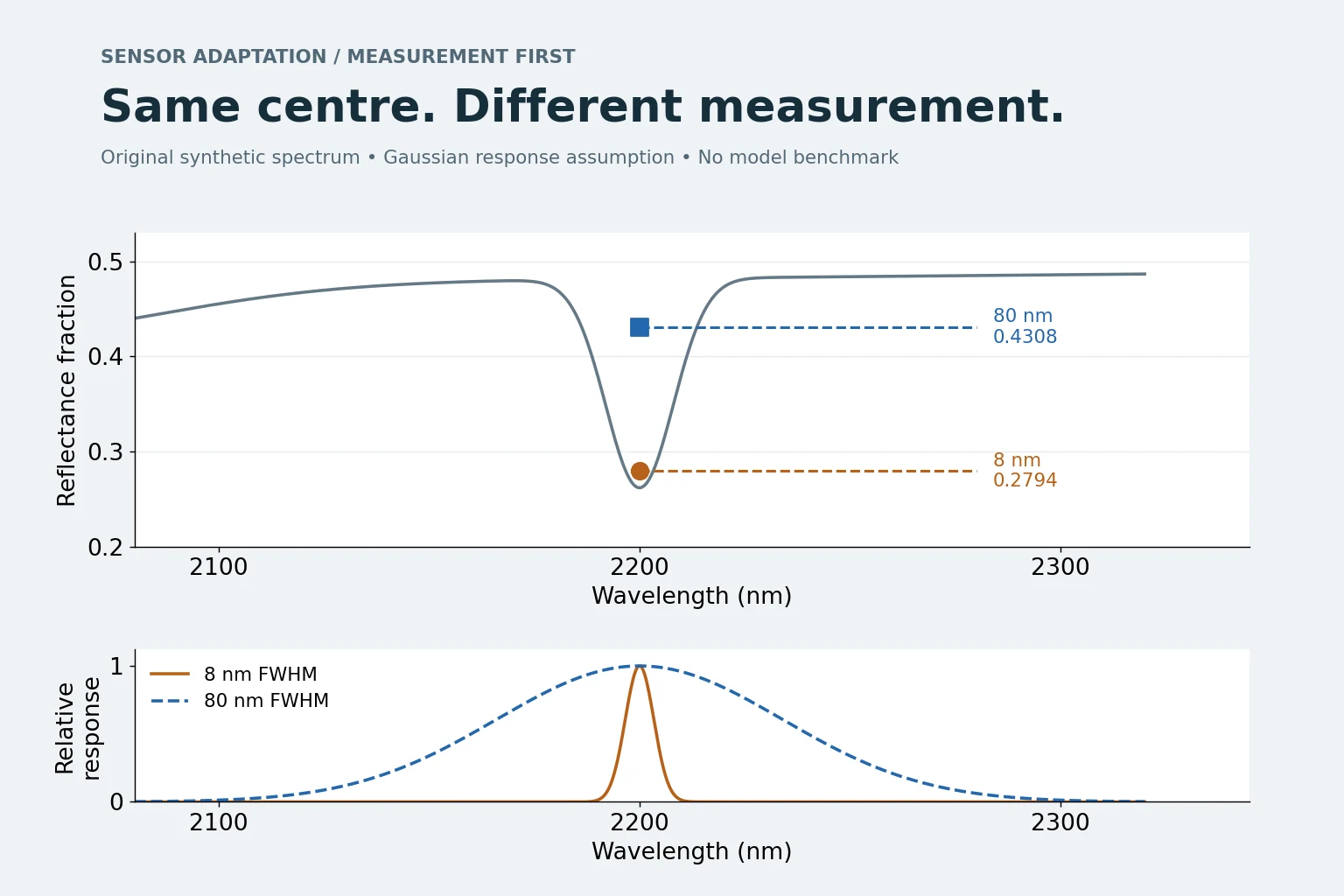
| 2200 | 2200 | 0.43079 | 0.27939 | 0.43110 | 100.00% |
| 2225 | 2225 | 0.44378 | 0.47976 | 0.44390 | 100.00% |
| 2250 | 2250 | 0.46588 | 0.48400 | 0.46576 | 100.00% |
| 2275 | 2275 | 0.47998 | 0.48500 | 0.47986 | 100.00% |
| 2300 | 2300 | 0.48517 | 0.48600 | 0.48513 | 100.00% |
Download runnable CPU source · Download Python notebook
Static default results shown. Enable JavaScript for controls; the Python download works independently.
Normalize units and audit response coverage
Convert wavelengths to one internal unit before aligning anything. In this lab the unit is nanometres: 2.2 micrometres is 2,200 nm. Convert both centres and widths, not only the wavelength axis. Confirm that reflectance fractions and percentages are not mixed. Radiance, reflectance and standardized network inputs are different quantities; an arbitrary min–max transformation does not provide radiometric calibration.
Check for finite wavelengths, duplicates, unsorted arrays, sentinel values and invalid intervals. If you intentionally sort wavelengths, carry the paired observations, responses and validity flags with them. A target band centred inside the source range can still extend outside it. Coverage must be evaluated over the target response, including its tails, rather than by testing the centre alone.
The lab requires at least 99.9% of the modeled target-response weight to lie in valid reconstructed support. It uses a Gaussian truncated at plus or minus four sigma, and normalizes only after that coverage check. The omitted Gaussian tail is approximately 0.0063% of the infinite response area. These are disclosed numerical choices, not a universal instrument-quality threshold. A rejected target stays unavailable; it is never filled with zero or extrapolated.
An invalid source channel blocks interpolation on both adjacent intervals. We therefore do not bridge the deliberately masked gap. In real data, use the delivered validity mask and a documented gap policy. Keeping a value just because an interpolation function returned a finite number is not a scientific coverage check.
Integrate a response instead of sampling a point
For this teaching model, a target band measures y_j = integral[r(lambda) S_j(lambda) d lambda] / integral[S_j(lambda) d lambda]. Here r is a synthetic reflectance curve and S_j is a nonnegative response. Normalization preserves a constant spectrum. Numerical integration needs interval widths: an unweighted sum on a nonuniform wavelength grid can overweight densely sampled regions.
This expression is a reflectance-domain approximation, not a universal radiometric forward model. Depending on product definitions, accurate processing may require irradiance weighting, detector calibration, atmospheric effects or other terms. The lab intentionally removes those complications so that the consequences of finite band width can be inspected directly.
Centre interpolation estimates a point-like value at the target centre. Response integration averages over an interval. Even a perfect sample of the underlying curve at the centre can differ from the band average around a narrow trough. In the broad-target preset, the exact synthetic centre samples have a mean absolute error of about 0.02977 reflectance fraction against the finite-band reference. This is an error in the operation, not an error in a neural network.
The browser computes composite midpoint quadrature using cells no wider than 0.5 nm. The downloadable Python implementation computes the same quantities independently. Both compare reference and estimates on an identical retained band set, and both expose per-band coverage and values. Those audit fields matter as much as the headline error.
Resampling cannot recover unmeasured detail
The source sensor does not provide the underlying continuous curve. It provides its own band-integrated observations. Connecting those band averages with a line is a reconstruction assumption. Integrating that reconstruction through a second response can be a useful approximation when the source response is sufficiently narrow and the sampling sufficiently dense for the relevant features, but it is not exact sensor conversion in general.
The lab deliberately shows this distinction. Its black target markers come directly from the known synthetic curve. Its blue estimates first measure the source bands, reconstruct between those measurements, then integrate the reconstructed curve. The small remaining default error reflects that extra approximation. The source measurements must not be silently treated as exact high-resolution point samples.
For ideal shift-invariant Gaussians on a continuous dense grid, two successive convolutions add their variances. Consequently, convolving an already broadened signal with the full target Gaussian adds blur rather than undoing the source response. A differential kernel can describe a restricted Gaussian broadening case when the target variance exceeds the source variance; it is not a general solution for irregular SRFs, missing channels or sparse data.
A request for bands narrower than the source resolution is an inverse problem. Many fine-scale spectra can give nearly the same coarse observations. A learned adapter may supply a useful prior, but a plausible output is not a recovered measurement. Label reconstructed or imputed channels and test their downstream consequences. Increasing the number of interpolated channels increases array length, not information.
Choose an adaptation route that matches the evidence
DOFA uses wavelength-conditioned dynamic patch embedding: band-centre metadata drives a hypernetwork that generates input projection weights for different band configurations. The paper provides a mechanism for handling varying channel counts and sensor inputs. That mechanism does not encode a complete measured SRF merely because it receives a centre wavelength. This guide cites the revised v3 paper, which also includes DOFA+. No reported benchmark score is reproduced here. [1]
SpectralEarth introduces EnMAP-derived pretraining data and models with a spectral adapter before conventional vision backbones. Its adapter uses spectral one-dimensional convolution blocks, and the study compares frozen-backbone, adapter-tuning and full-tuning evaluation settings. The v2 paper’s preprocessing retains 202 bands after specified exclusions. Those design and evaluation choices motivate useful experiments; they do not establish that an arbitrary new sensor is compatible without checking the released implementation. [2]
In practice, consider a native wavelength-aware input route, a fixed physically justified common-band representation, or a learned target-sensor adapter. Each answers a different problem. A common representation may discard useful wavelengths. A learned adapter consumes target training data and may overfit. A flexible input layer can avoid a fixed channel-count constraint while remaining sensitive to calibration and distribution shift. Select among them using a controlled target-domain comparison.
Audit pretraining provenance before claiming transfer
Identify the precise pretraining dataset release, sensor mix, acquisition periods, geographic coverage, preprocessing and initialization lineage documented for the checkpoint. Keep the paper version separate from the actual weight release: later manuscript revisions need not describe every earlier downloadable checkpoint. Record license and redistribution requirements before packaging model assets.
Check whether downstream scenes, nearby overlapping footprints, repeated acquisitions of the same location or derived products could have appeared in pretraining. A spatially disjoint supervised train/test split does not by itself rule out pretraining exposure. If scene lists are incomplete, report that overlap could not be ruled out. Do not turn missing provenance into a claim of strict zero-shot geographic generalization.
Define what transfer means in the report. New labels on familiar imagery, a new acquisition date, a new region and an unseen sensor are distinct experiments. Record which changed and which remained shared. If adapting with unlabeled target test imagery is part of the protocol, describe it as transductive adaptation and compare against baselines with equivalent access; do not present it as a purely inductive holdout.
Fit adapters and statistics on training data
Create the evaluation split before fitting normalization, imputers, dimensionality reduction, calibration mappings or learned adapters. Use training observations to estimate their parameters, validation data to select hyperparameters, and an untouched test set for the final chosen pipeline. Fitting a scaler on all pixels still leaks target-distribution information even when no labels are used.
Choose split units that reflect the deployment claim, such as independent scenes, fields, sites or acquisition campaigns. Keep overlapping patches and their spatial context together; add a justified separation buffer when neighbouring context could cross the boundary. For paired sensors, keep both measurements of the same physical sample in the same split. Otherwise a cross-sensor experiment can quietly become a same-sample recognition task.
For adapter-only training, state exactly which parameters and buffers can change. Freezing gradients on the backbone is not sufficient if batch-normalization running statistics continue updating. Specify training/evaluation modes, normalization-buffer treatment and any updated head. Save the list of trainable modules and parameter count with the run. An adapter-plus-head experiment should be named that way rather than implying that only one component changed.
Unit-test the data boundary. Changing test labels must not change fitted preprocessing or adapter weights. Reordering test batches should not silently refit statistics. A fitted pipeline should transform held-out observations without calling fit again. The spatial split guide and reproducible pipeline guide cover these broader safeguards.
Compare models under a shared protocol
Use the same train/validation/test units, label budget, target coverage and evaluation mask across candidate adaptation strategies. Start with a simple target-sensor baseline. Add a frozen pretrained encoder with a training-fitted head, an explicitly defined adapter-plus-head setting, and full fine-tuning only if the available data and compute justify that comparison. Include a comparable random-initialization baseline when asking whether pretraining helped.
Separate source-only transfer from target-supervised adaptation. They use different information and should not share an unlabeled performance heading. Report the number of target labels, optimization budget, seeds and model-selection rule for each method. Keep physical band harmonization fixed when isolating a training strategy; keep the learning strategy fixed when isolating a harmonization choice.
Report task-appropriate per-class and aggregate metrics, errors by sensor/site/date, retained sample counts, and variation across independent runs or evaluation units. Repeated random pixels from one scene are not independent geographic replications. Revisit both accuracy and uncertainty under the target distribution. A change in reconstruction error does not imply a corresponding improvement in classification or segmentation.
Run the six measurement experiments
1. Narrow source to broad target: source FWHM 8 nm, centre spacing 5 nm, target FWHM 80 nm. All 13 target bands pass coverage. The response-resampling mean absolute error is approximately 0.000112, compared with 0.023902 for centre interpolation. The improvement is specific to this known synthetic curve and these measurement assumptions.
2. Centre values miss the band average: increase target FWHM to 120 nm. Response-resampling error is approximately 0.000041; centre interpolation is approximately 0.028146. The interface also reports the error of ideal centre samples taken directly from the synthetic truth. That extra diagnostic separates the point-versus-average mistake from source-sensor limitations.
3. Broad source to narrow target: source FWHM 100 nm and target FWHM 12 nm. Response resampling now has mean absolute error approximately 0.024944. The source trough was already flattened. A denser target grid or a different output channel count cannot undo that loss.
4. Sparse samples miss the trough: source spacing 60 nm and target FWHM 20 nm. The 2,200 nm narrow feature falls between source centres. The response estimate has maximum absolute error approximately 0.140880. A smooth line through the available channels is not evidence that the underlying spectrum was smooth there.
5. Missing coverage stays missing: mask source centres from 2,150 to 2,250 nm. Only two of the thirteen target bands meet the common-coverage rule. Rejected bands remain unavailable. Comparing this subset’s small error with the full-spectrum default would reward removal of the difficult region, so the retained count is displayed prominently.
6. Wrong wavelength metadata: shift true target centres by 20 nm while both estimators still use nominal centres. Response resampling now has mean absolute error approximately 0.023663. The mismatch is intentional. Real target truth would not normally be known; this synthetic experiment makes metadata sensitivity observable without pretending to estimate calibration uncertainty.
Reproduce the lab on a CPU
Download and extract the CPU source ZIP. With Python 3.10 or newer, run python python/sensor_adaptation.py from the extracted directory, then run python -m unittest discover -s tests -p "test_*.py". The core program and Python tests use only the standard library. They write results.json and one CSV per preset into an outputs directory. No model download, paid API, GPU or network connection is needed.
The notebook repeats the measurement definition, runs every preset, checks units and constant-preservation, inspects missing support, and compares narrow-to-broad with broad-to-narrow conversion. JupyterLab is an optional interface dependency; the numerical implementation itself has none. The notebook embeds its numerical implementation, so the notebook download also works on its own. Every code cell is executable in order, and the package also includes a sequential-cell runner for CPU environments without Jupyter.
The JavaScript implementation powers the live controls rather than selecting precomputed error labels. The downloaded run JSON contains the settings, source samples, target values, metrics and stated assumptions. The CSV contains the per-band numbers. Copy experiment link preserves only allowlisted numerical settings and the selected coverage mode, so another reader can reproduce that state.
The downloadable tests verify constant preservation, symmetry, finite bounds, no extrapolation, gap rejection, preset counterexamples and agreement between Python and JavaScript. An additional author-side SciPy quadrature check compares the integration routine with an independent implementation; it is a numerical oracle, not validation of a real sensor.
Keep uncertainty and coverage separate
Response coverage is a fraction of modeled support, not a probability that the prediction is correct. The lab’s MAE and maximum error are deterministic discrepancies against known synthetic truth. They do not estimate confidence intervals, sensor noise, atmospheric-correction error or epistemic uncertainty in an encoder. Their precision should not be mistaken for physical accuracy.
For real adaptation, separate metadata uncertainty, measurement noise, preprocessing sensitivity, training variation and out-of-domain behavior. Test plausible centre shifts or response alternatives when calibration documentation supports those ranges. A sensitivity sweep is still conditional on the chosen alternatives; it does not become a confidence interval unless the underlying probabilistic assumptions are justified.
Wavelength overlap cannot resolve changes in spatial footprint, viewing geometry, atmospheric residuals or class prevalence. These can dominate after spectral harmonization. If a task requires a missing diagnostic wavelength, a model may learn a correlated proxy in the training domain and fail when that correlation changes. Evaluate the new sensor on the actual intended deployment conditions and retain an abstention or review route where consequences justify it.
A release checklist for a new sensor
Before reporting success, preserve the source and checkpoint manifests, exact weight hash, measured or assumed SRFs, validity masks, resampling implementation and numerical tolerances. Verify a constant-spectrum test, a narrow-feature counterexample and a known missing-gap case. Inspect several real preprocessed spectra and spatial patches before launching training.
Then save split identifiers, train-fitted transformations, updated parameter and buffer names, target-label budget, seeds, environment versions and the final selection rule. Check that all methods see the same eligible examples and that test data were not used to tune the pipeline. Archive per-unit metrics so an average cannot conceal one failing sensor or site.
The conclusion should match the evidence: the input contract passed, a specified adapter was trained on specified data, and a defined held-out evaluation produced a measured result. If only the synthetic resampling lab was run, the defensible conclusion is narrower: the implementation illustrates why bandpass, sampling and coverage matter. A tensor with the right number of channels is only the beginning.
Frequently asked questions
Does a variable-channel model make sensors interchangeable?
No. Input flexibility addresses a software and architecture constraint. Calibration, spectral response, coverage, spatial resolution and distribution shift still need independent checks.
Are centre wavelength and FWHM enough to reconstruct an SRF?
Only after adding a response-shape assumption. The lab uses an idealized Gaussian; measured responses are preferable when available.
Can interpolation recover narrow bands from broad ones?
It can produce more numbers, but it cannot uniquely recover unmeasured fine detail. A learned reconstruction adds prior assumptions that require validation.
Does this lab evaluate DOFA or SpectralEarth?
No. It evaluates original synthetic measurement and resampling operators. The two papers inform the guide’s architecture discussion; no foundation-model inference or fine-tuning is performed.
Why are some target bands unavailable?
Their response overlaps unsupported source wavelengths or masked interpolation intervals. The lab requires at least 99.9% modeled response coverage and never extrapolates or bridges missing neighbours.
Do I need a GPU or paid service to reproduce this?
No. The Python core and tests use the standard library on a CPU. JupyterLab is optional for opening the notebook, and no model weights or external data are downloaded.
References and further reading
- Xiong et al. Neural Plasticity-Inspired Multimodal Foundation Model for Earth Observation (DOFA), arXiv:2403.15356v3, 2025 revision, methodology §§3.2–3.3.
- Ait Ali Braham et al. SpectralEarth: Training Hyperspectral Foundation Models at Scale, arXiv:2408.08447v2, 2025 revision, preprocessing, architecture and evaluation protocols.
- EnMAP-Box official documentation. Spectral resampling to wavelength: linear interpolation and nearest neighbour.
- EnMAP-Box official documentation. Spectral resampling to wavelength and FWHM.
- EnMAP-Box official documentation. Spectral resampling to custom sensor: explicit responses and Gaussian/FWHM approximation.
- EnMAP-Box official documentation. Spectral resampling to response function library.
Reader feedback
Reads since 1 October 2026: at least 15 seconds with the article visible, counted once per browser per day. Reactions are anonymous and can be changed.
Loading reader feedback…
Discuss this article
Ask a technical question, challenge an assumption or share evidence from your own work.