
One command should leave a result you can explain
An HSI result becomes easier to trust when its inputs, split, learned transformations and evaluation can be inspected together. A notebook that ends with an accuracy score leaves too much implicit. Which wavelength order was used? Which pixels fitted the scaler? Was the plotted prediction evaluated on the same mask? Could someone reload the saved model and obtain the same labels?
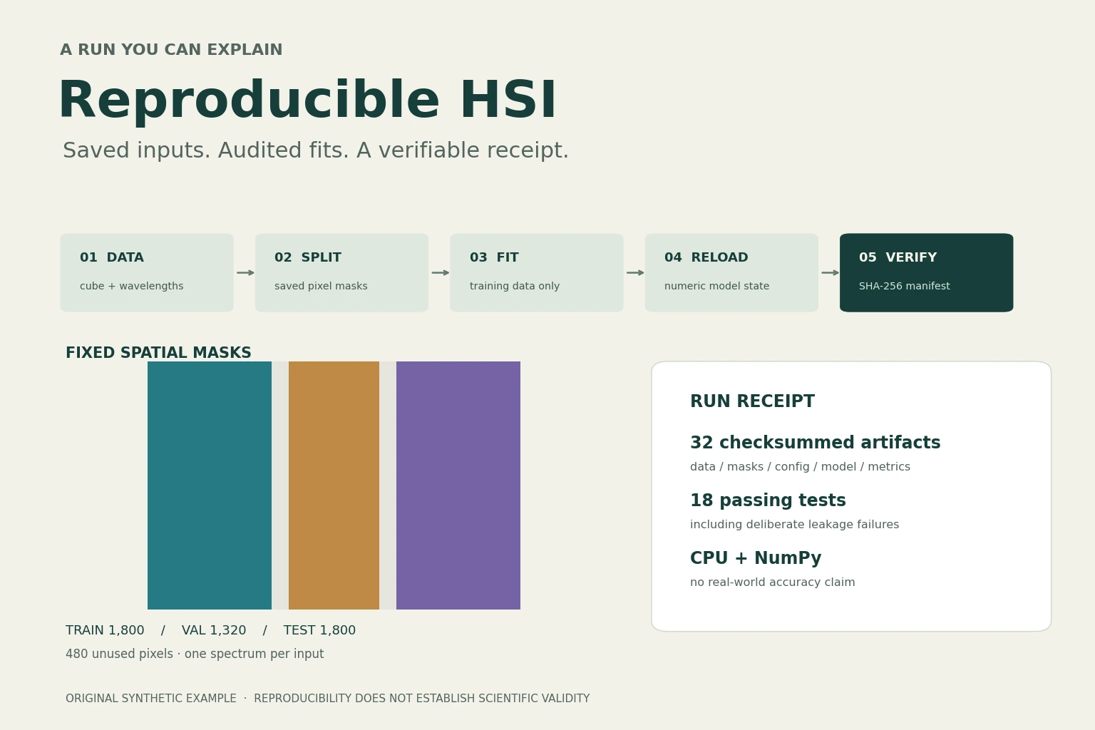
This capstone builds a small CPU pipeline that answers those questions with files and tests. It generates a synthetic hyperspectral cube, saves fixed spatial masks, fits a simple training-only baseline, reloads its numerical state, computes held-out metrics and writes a checksummed run manifest. The download includes the runnable module, tests, notebook, configuration and a complete example run. NumPy is the only core dependency.
The preprocessing guide, spatial-split guide and fine-grained metrics guide explain the individual choices in depth. Here the focus is connecting them into an auditable workflow. All spectra, labels and scores below are generated teaching examples; they do not reproduce a published experiment or measure performance on a real sensor.
Separate rerun consistency, portability and scientific validity
Start by writing the claim your checks actually support. In this release, two executions on the tested environment produced byte-identical recorded artifacts. That is a useful regression check: an unexpected difference deserves investigation. It does not show that another operating system, CPU, library build or future release must produce identical bytes.
NumPy documents strict conditions for random-stream compatibility, including the generator, seed, call sequence, build, environment and machine. The example explicitly constructs Generator(PCG64(seed)) rather than relying on a process-global random state. Saving generated arrays also gives a future reader an exact input even if regeneration changes. A seed is one part of the record. [1]
Scientific validity is a separate question. A perfectly repeatable pipeline can use wrong labels, select a model with test feedback or evaluate neighbouring pixels as though they were independent sites. Reproducibility makes those choices inspectable; it cannot make them appropriate. For a portability check, compare meaningful arrays and metrics using justified tolerances, investigate changed predictions and document the observed differences rather than promising universal bitwise equality.
Sources: [1]
| Check | Evidence in this example | Limit |
|---|---|---|
| Input identity | SHA-256, shape, dtype, wavelength axis and class mapping | A checksum cannot establish physical calibration or label truth |
| Split membership | Boolean masks, unused pixels, counts and pixel IDs | Disjoint regions need not be independent scenes |
| Fit boundary | Training-only statistics and holdout-perturbation tests | Does not detect informal test-set tuning |
| Model persistence | Numeric state reloaded before saved predictions | Only the supplied model layout is supported |
| Evaluation identity | Prediction IDs, confusion counts and explicit macro policy | Synthetic scores do not establish application performance |
| Rerun consistency | Two byte-identical runs in the tested environment | No cross-platform or cross-version bitwise guarantee |
| Artifact integrity | Manifest verification and a deliberate tamper test | An unsigned manifest does not authenticate its publisher |
Define the input contract before flattening the cube
The default cube has shape (60, 90, 41): row, column, band. Wavelengths run from 900 to 1700 nm in 20 nm steps. Values are dimensionless reflectance-like numbers, not calibrated observations. Three arbitrary labels, Class A, B and C, identify generated spectral families. The small repeated inclusions only make the map easier to inspect; they do not represent known physical objects.
Validation requires finite floating-point spectra, an aligned integer label image, a positive strictly increasing wavelength vector and an aligned nonempty boolean band mask. Descending or duplicated wavelength coordinates raise an error. For real data that need reordering, apply one verified permutation to both spectral columns and their metadata upstream. No array check can detect a plausible-looking but already mislabelled wavelength axis without independent metadata.
Three deliberately contaminated bands at 1340, 1360 and 1380 nm are excluded. This mask is known from the generator, so it does not learn from the held-out region. The positions are an example, not a recommendation for any instrument. There is no spectral interpolation, smoothing, derivative, PCA or spatial filter in this baseline; those additions would each need their own recorded parameters and tests.
Runnable CPU reference · all data are synthetic
Inspect a complete run receipt
Follow generated data through saved masks, training-only fitting, reloaded predictions and integrity checks. The notebook and command-line script share the same implementation.
The notebook imports the adjacent Python module: extract the full ZIP before running it. Tested with CPython 3.12.14 and NumPy 2.3.5. No GPU or dataset download is needed.
python -m unittest -v test_pipeline.py
python hsi_pipeline.py run --config config.json --out my-run
python hsi_pipeline.py verify --out my-run
Use a new output directory for each run. The script refuses to overwrite an existing one.

1. Verify the input identity
The cube is float64 with shape (60, 90, 41). Its axis order is row, column, band. The wavelength range is 900–1700 nm. Bands 1340, 1360 and 1380 nm are excluded because the generator deliberately corrupts them. This is not a sensor-specific masking recommendation.
Cube SHA-256: 250a9397c3869c0b3b93c72ce3483f2577a5b083e613ffaa13df0c7ad6ed55aa
2. Check the split and fit boundaries
All three masks are boolean and non-overlapping. The scaler and centroids use the 1,800 training pixels only. Validation is diagnostic; no hyperparameter selection or refit occurs. The input is one pixel spectrum, with no spatial filtering or patches.
Training-mask SHA-256: 1bb688914e9b3da4b205cc0e72ea2bcbaf3ed3ed70b9a684baa26abf5d9e24c5
The tests deliberately alter held-out spectra and labels and require every fitted array to stay unchanged. A separate test replaces the mean with an all-pixel mean and requires the audit to reject it.
3. Read the saved held-out counts
These counts are synthetic regression fixtures. Reference classes are rows; predictions are columns. No measured HSI performance claim is made.
| Reference | Predicted A | Predicted B | Predicted C |
|---|---|---|---|
| Class A | 591 | 45 | 0 |
| Class B | 0 | 582 | 0 |
| Class C | 0 | 0 | 582 |
OA = 0.975. Macro-F1 = 0.975368. All three classes have reference support. Undefined ratios are null; macro metrics exclude reference-absent classes and list them explicitly.
Download the full metric definitions and per-class values · Open the confusion figure

4. Inspect what the manifest proves
The manifest records file hashes and sizes; numeric arrays also record shape and dtype. It covers data, masks, configuration, environment, fitted state, predictions, evaluation, figures and the exact executed source. It does not hash itself.
Source SHA-256: f2d06edc304fe894519cc52e15517f5b40f74badfdeec4bdb6740882ebd5f5d9
Matching hashes establish agreement with this manifest. An unsigned manifest does not authenticate the publisher, and a reproducible run can still have an invalid evaluation design.
Verification scope: 18 Python tests, model-reload agreement, independent scikit-learn numerical checks, and two byte-identical local reruns. Notebook cells were executed sequentially in Python; no Jupyter kernel was used. Cross-platform bitwise agreement is not promised.
Save split masks as experimental inputs
The training region uses zero-based columns [0, 30), validation uses [34, 56), and test uses [60, 90). A half-open interval includes its first column and excludes its last. The resulting counts are 1,800 training, 1,320 validation, 1,800 test and 480 unused pixels. The two four-column gaps remain visible and are never silently reassigned.
The validator rejects overlapping, empty, non-boolean or misaligned masks. Each mask is saved independently, along with class counts and an explicit unused-pixel mask. Training must contain every configured class. Pixel IDs use row-major order: row × width + column. Saving the IDs beside prediction vectors prevents a later reshape or sorting change from attaching a prediction to the wrong location.
This example consumes one pixel spectrum at a time, so its input-support radius is zero. The four-column gaps illustrate mask bookkeeping; they are not a demonstrated decorrelation distance. Patches, spatial smoothing and overlapping acquisitions change the relevant support. Follow the spatial-split guide when designing those boundaries, and use independent acquisitions when the claim concerns new scenes or sensors. One synthetic scene cannot establish that claim.
Make the fit boundary small enough to audit
The fitting function selects cube[train_mask] before learning any statistics. It retains the fixed good-band columns, calculates each band's training mean and population standard deviation, and standardises the training spectra. A near-constant band receives scale 1 when its standard deviation is at or below the recorded floor of 1e−12. The same saved mean, scale and band order are applied at prediction time.
The model is an ordinary nearest-centroid baseline: average the standardised training vectors in each class, then predict the closest centroid by squared Euclidean distance. Exact ties choose the lowest configured class ID. It has no random optimiser, epochs or hidden checkpoint-selection rule. Its simplicity makes state inspection practical; it is not a recommendation that every HSI problem should use this classifier.
Learned preprocessing must stay inside the training boundary, including when it does not use class labels. The scikit-learn documentation explains this failure mode for scaling, imputation, feature selection and PCA and recommends pipelines for consistent fold-local fitting. The reference here implements the small calculation directly so its saved arrays can be read without deserialising a library estimator. [2]
Two checks target the boundary. First, changing every validation and test spectrum and label leaves the fitted means, scales and centroids unchanged. Second, an audit recomputes training statistics and checks the stored fit pixel IDs; a deliberately global-fitted mean fails. These tests expose specific implementation mistakes. They do not prove that an experimenter never inspected held-out information elsewhere.
Sources: [2]
Freeze the recipe before reading test results
The configuration is pre-specified. Validation is reported as a diagnostic, with no search, automatic selection or refit. Test evaluation happens after the fixed model has been fitted and reloaded. If you add model selection, record the candidate configurations, choose with validation or inner folds, and reserve a separate final test. Each fold needs its own fitted preprocessing state.
The example saves confusion counts with reference classes as rows and predictions as columns, plus OA, per-class precision, recall, F1 and IoU. Macro-F1 and mean IoU average classes with positive reference support. An undefined ratio is null, and unsupported class IDs are listed. For example, a present class with no correct predictions receives F1 zero; a class absent from both truth and prediction has undefined F1. The separate metrics guide discusses why the support and averaging policy matter.
In the tested default run, the 1,800 test pixels produce rows [591, 45, 0], [0, 582, 0] and [0, 0, 582]. OA is 0.975 and macro-F1 is approximately 0.975368. These numbers are frozen regression fixtures for generated data. They should help detect a changed implementation, not become targets to improve by altering the test recipe. No confidence interval or real-world generalisation claim is attached to them.
Reload the exact state used to make predictions
A saved label map cannot answer how a model would predict another input. The model directory therefore contains training means, scales, class centroids, class order, the original wavelength axis, the retained-band mask, fit pixel IDs and the scale-floor setting. A small JSON file explains the distance, tie rule and standard-deviation convention.
All arrays are numerical .npy files saved and loaded with allow_pickle=False. NumPy warns that loading pickled object arrays can execute code; avoiding object serialisation is appropriate for this small reference. This is not a general-purpose security guarantee for arbitrary downloaded files. Verify a trusted release and avoid loading files whose origin you cannot establish. [3]
The run reloads the numerical state before calculating its stored predictions and checks agreement with the in-memory model. Prediction also rejects any changed wavelength axis. A same-shaped input with different band coordinates must not slip through because its matrix dimensions happen to match. The model package is intentionally specific to this teaching layout rather than a universal exchange standard.
Sources: [3]
Give every important artifact a place in the manifest
The run contains data, masks, fitted state, prediction vectors, pixel IDs, metric definitions, two figures, configuration, a compact environment record and a snapshot of the executed source. The manifest lists 32 files with SHA-256 digests and byte sizes; numerical arrays also include shape and dtype. It is written last as a completion marker and does not attempt to hash itself.
Verification recalculates each digest, rejects missing or extra files, and reports a mismatch if even a whitespace byte changes in a recorded JSON file. This checks integrity against the manifest. It does not authenticate the author: someone who changes both an artifact and an unsigned manifest can make them agree. For a release, keep the archive digest or signature in a separately trusted record.
The environment record names Python, NumPy, operating system and machine architecture without dumping environment variables or secrets. The dependency file pins the tested NumPy version, but it is not a complete cross-platform environment lock. A larger study may also need wheel hashes, a container digest, numerical-library builds, drivers, accelerator settings and a release or commit identifier. Keep run timestamps in the experiment record; deterministic artifact comparison should not confuse changing clock metadata with changed numerical results.
Write tests for mistakes you expect people to make
The included 18 tests cover failure paths as well as a successful run. Known small fixtures check the training statistics, nearest-centroid predictions, exact-tie rule and a hand-computable confusion matrix. Independent checks also compare the release's standardisation and metrics with scikit-learn. A checksum test deliberately changes a saved file and requires verification to fail.
The test suite also generates two complete runs in separate temporary directories and compares their manifests. That verifies the same-environment byte-identity claim for this release. The notebook imports the same module, so it is an explanation of the pipeline rather than a second implementation that can drift. Its code cells were executed in order in a fresh Python namespace; this check did not launch a Jupyter kernel.
Tests cannot enumerate every error. They are especially valuable when their assumptions are visible: this package has complete finite inputs, three known classes, pixel-only support and a fixed training protocol. Real missing data, a new class map or patch-based inputs require deliberate extensions rather than removing validation until the code runs.
Run the bundle in a clean directory
Download the complete CPU reference bundle and extract it. The tested environment was CPython 3.12.14 with NumPy 2.3.5 on Linux x86_64. Create and activate an environment using your platform's usual commands, then install requirements.txt. The README gives the exact sequence and the notebook provides a guided walkthrough.
From the extracted folder, run python -m unittest -v test_pipeline.py, then python hsi_pipeline.py run --config config.json --out my-run, and finally python hsi_pipeline.py verify --out my-run. The output directory must be new. Reusing an existing one raises an error so a fresh run cannot silently overwrite an earlier receipt.
Start by inspecting config.json, the split summary, model.json and evaluation/test_metrics.json. Then open the two SVG figures. The prediction map shows only the test stripe, with the rest grey; the reference map is explanatory context. Check that the mask counts, prediction count and confusion-matrix total agree before interpreting the score. No GPU, credentials, model download or external dataset is required.
Carry the same contract into a PyTorch experiment
A neural model adds more state, but the input, split and evaluation obligations remain. PyTorch's reproducibility documentation describes seeding its random generator, controlling other libraries' generators and using deterministic algorithms where available. DataLoader worker seeding and generator handling need attention as well. Deterministic operations can have a performance cost. [4]
The same documentation explicitly warns that identical seeds do not guarantee identical results across PyTorch releases, platforms or CPU and GPU execution. Do not turn a few flags into a universal reproducibility claim. Record the actual framework, device, numerical precision, relevant backend settings, data order and checkpoint-selection policy, then test the particular run you plan to report. [4]
For resumable training, also preserve optimiser and scheduler state, random-generator state and the position in the data stream. A model-weight file alone does not describe where training stopped. This reference deliberately stays on the CPU and does not install or execute PyTorch; these are extension considerations, not checks claimed for the supplied code.
Sources: [4]
Finish with a release another researcher can understand
Sandve and colleagues' rules for reproducible computational research encourage tracing results to their inputs and preserving the software and intermediate work needed to recreate them. Here, the manifest and exact source snapshot put that idea into a small inspectable form. In a real study, connect the receipt to the original acquisition records, annotation provenance and the paper's experiment description. [5]
Barker and colleagues describe FAIR4RS as principles for making research software findable, accessible, interoperable and reusable. Version-specific identification, metadata, provenance and an explicit reuse licence all matter. A ZIP, tests and a checksum alone do not establish complete FAIR4RS compliance. This educational release does not claim that status; the publisher should select a licence and archive a citable version before presenting it as a reusable research-software release. [6]
The practical stopping point is simple: a colleague can start from the recorded inputs, run the stated command, inspect the same split and fitted state, and explain any difference in the outputs. That is a strong foundation for the next experiment. Its scientific claims still depend on measurements, labels, sampling and an evaluation design that match the intended use.
- Preserve input units, axis order, class mapping and data provenance
- Save masks and pixel IDs before fitting; inspect independence at the appropriate scale
- Keep every learned transformation inside its training fold
- Record selection rules and leave the final test outside development feedback
- Reload the saved model and verify both its predictions and artifact hashes
- Publish exact tested versions, clear limits, source attribution and an intentional reuse policy
Frequently asked questions
Is setting a random seed enough for reproducibility?
No. Preserve the input data, split, source, configuration, fitted state and environment. A seed alone does not guarantee cross-platform or cross-version numerical identity.
Does the Python example require a GPU or an HSI dataset download?
No. It generates a small synthetic cube and runs with NumPy on the CPU. The download includes an example run and its saved arrays.
Why keep a validation mask if the model is fixed?
It makes the roles explicit and provides a diagnostic report. This example performs no model selection or refit. If selection is added, use validation or inner folds and preserve a separate final test.
Does a passing checksum prove that a result is scientifically valid?
No. It verifies agreement with a manifest. Correct measurements, labels, sampling, independence and evaluation still need separate evidence, and an unsigned manifest does not authenticate itself.
Why does the pipeline refuse an existing output directory?
Each run should leave its own receipt. Refusing reuse prevents a new execution from silently replacing an earlier experiment's artifacts.
Can I replace the nearest-centroid model with PyTorch?
Yes, as an extension. Retain the input, split, preprocessing and evaluation contracts, then record and test the additional random, backend, training and checkpoint state. PyTorch is not used by this CPU reference.
References and further reading
- NumPy Developers. Random generator compatibility policy.
- scikit-learn Developers. Common pitfalls: data leakage and consistent preprocessing.
- NumPy Developers. numpy.load: numerical arrays and the allow_pickle security warning.
- PyTorch Contributors. Reproducibility: random seeds, deterministic algorithms and platform limits.
- Sandve, Nekrutenko, Taylor and Hovig (2013). Ten Simple Rules for Reproducible Computational Research. PLOS Computational Biology 9(10), e1003285.
- Barker, Chue Hong, Katz and colleagues (2022). Introducing the FAIR Principles for research software. Scientific Data 9, 622.
Reader feedback
Reads since 1 October 2026: at least 15 seconds with the article visible, counted once per browser per day. Reactions are anonymous and can be changed.
Loading reader feedback…
Discuss this article
Ask a technical question, challenge an assumption or share evidence from your own work.