
Start with an eligible reference, then calculate similarity
A spectral library is a collection of measurements linked to sample descriptions. It becomes useful for identification when a reference and an observation are comparable in physical quantity, wavelength coverage, measurement response and sample condition. A nearest-neighbour search can always return a winner from a nonempty library. The scientific question is whether that winner is an adequate explanation of the observation.
This guide follows a single-spectrum workflow: audit the reference, put it into the sensor’s measurement space, compare several candidates and decide how much the result supports. It does not estimate material fractions. The mixed-pixel unmixing guide addresses that separate inverse problem. Here, even a nominally single-material observation can be ambiguous because the right reference is missing, two candidates look similar, or the comparison has discarded the distinguishing feature.
The interactive lab makes those failure modes inspectable. Every curve is an original mathematical construction named A, B or C. None is a measurement of a mineral, crop, polymer or other material. The known generating curve is A, which lets us test whether the matching procedure recovers its source under deliberately changed conditions.
Use the library documentation as part of the data
The USGS Spectral Library Version 7 includes laboratory, field and airborne spectra, with sample and measurement documentation. Its report describes instrument effects, wavelength sampling and bandpasses, and versions convolved or resampled for selected sensors. Keep the exact release and spectrum identifier with the data; a material name by itself does not identify one measurement. [1]
The ECOSTRESS Spectral Library, formerly the ASTER library, combines contributions from JPL, Johns Hopkins University and USGS–Reston. Its website links the measurement descriptions for its constituent collections. This means that a shared download portal should not be treated as evidence of one uniform acquisition protocol. Read the ancillary record and the appropriate collection description before pooling entries. [2]
For real work, save a small manifest containing the library release, sample identifier, source URL, retrieval date, file checksum, original quantity and units, preprocessing steps and reuse terms. Preserve the source files separately from derived sensor-ready vectors. The USGS data-release page marks that release CC0; the ECOSTRESS site carries a Caltech copyright notice and requests scholarly attribution. Check the terms for the particular assets you redistribute. This article embeds neither library’s measurements or imagery. [3, 2]
| Score | Direction | What to keep in mind |
|---|---|---|
| Cosine similarity | Higher is closer; dimensionless | Invariant to positive scaling; undefined for zero vectors |
| SAM | Lower is closer; degrees in this lab | Monotonic transform of cosine, not an independent vote |
| Euclidean distance | Lower is closer; fractional-reflectance or ratio scale | Sensitive to amplitude, band count and units |
Audit sample condition and measurement geometry
A material label is only one part of a useful reference record. Record particle-size fraction, sample preparation, moisture or drying condition where documented, purity or accessory constituents, surface presentation and the measurement date. Treat an undocumented field as unknown. Avoid silently converting “not reported” into “dry,” “pure” or “representative.”
The JPL collection description explicitly includes grain-size series, ancillary mineral information and purity evaluation by X-ray diffraction. It also describes hemispherical reflectance measurements and the sample preparation used for that collection. The JHU documentation distinguishes measurement types and describes directional-hemispherical measurements and instrument joins. These are concrete reasons to retain provenance at spectrum level. [4, 5]
Before matching, ask whether the observation is a powdered laboratory sample, a leaf, a canopy or a remotely viewed surface. Illumination angle, viewing direction and collection geometry affect what “reflectance” means operationally. A carefully calibrated spectrum can still describe a different measurement configuration from the target. Exclude clearly incompatible entries or report them as analogues, and test plausible condition variants rather than selecting only the most convenient reference.
Interactive · synthetic reference matching
When the closest curve changes
Curve A generated the query. Change the comparison and see which eligible reference wins. A, B and C are invented curves with no physical material identities.
Only eligible references are plotted. Identical curves overlap; the query is drawn on top. Band centres are connected for readability.
Closest candidate A across 37 bands. Best SAM: 0.0000°. This is a similarity result within the supplied library, not proof of material identity.
| Candidate | SAM ↓ | Cosine ↑ | Euclidean ↓ |
|---|---|---|---|
| A · twin troughs | 0.0000° | 1.000000 | 0.0000 |
| C · darker look-alike | 1.1933° | 0.999783 | 1.0086 |
| B · shifted trough | 3.7370° | 0.997874 | 0.1890 |
37 bands. Euclidean distance uses reflectance fraction. Cosine is dimensionless; SAM is in degrees. Sorting: lowest SAM first.
Runner-up gap: 1.193259° on the selected score scale. This is not a probability or validated acceptance test.
Measurement and preprocessing controls
Gaussian responses are truncated at ±3σ and renormalized. The query always uses SRF integration. The reference method applies to every candidate. Continuum removal follows band integration and window selection.
Static exact-reference example. Enable JavaScript to change settings.
No material identification, confidence probability or acceptance threshold is validated here. All calculations stay in your browser; no data is uploaded.
Make units and missing bands explicit
Use a canonical wavelength unit in the computation. One micrometre equals 1,000 nanometres, so 2.2 µm and 2,200 nm must address the same location. If an input is given as wavenumber in cm⁻¹, use wavelength in µm = 10,000 / wavenumber, then sort the resulting wavelengths and carry the paired values with them. A uniform wavenumber grid becomes a nonuniform wavelength grid.
For reflectance, convert 35 percent to 0.35 before an amplitude-sensitive comparison. Both descriptions represent the same ratio. Radiance, reflectance, emissivity and pseudo-absorbance are different quantities; matching their array lengths does not make them interchangeable. Record transformations and their assumptions. The reflectance calibration guide explains the reference-measurement step that precedes this comparison.
Check that wavelengths are finite, strictly increasing after any intentional reordering, and paired one-to-one with values. Detect duplicates and sentinel values before interpolation. In the USGS ASCII release, deleted channels use −1.23 × 10³⁴; treating that number as a real reflectance would corrupt a norm or a resampled band. [6]
Use one declared comparison band set for every candidate in a ranking. If each candidate gets a different favourable subset, the scores no longer answer the same question. Missing coverage must remain missing: do not extrapolate beyond a reference’s support or interpolate across a known invalid spectral gap merely to obtain a complete matrix.
Sources: [6]
Match the band response, not just its centre
A sensor band responds over an interval. For this tutorial’s reflectance-domain approximation, its band value is rᵢ = ∫ r(λ) Sᵢ(λ) dλ / ∫ Sᵢ(λ) dλ, where Sᵢ is a nonnegative response function. The normalization preserves a constant spectrum. Real radiometric processing may additionally require illumination or irradiance weighting and the instrument’s calibration definition; the simple expression is not a universal forward model.
Interpolation at the band centre evaluates one point. Response integration averages across the band. Those operations differ most visibly around a narrow absorption. If a Gaussian response is assumed from an FWHM, state that approximation; use measured spectral response functions when available. ENVI’s resampling documentation distinguishes inputs consisting of centres, centres plus FWHM, and explicit filter functions. [7]
The lab generates the observation by integrating A through a Gaussian response. Its references can use that same response or a deliberately mismatched centre-only sample. With the 160 nm FWHM preset, centre-only A has a nonzero spectral angle despite being the generating curve. Returning the reference method to “Match the SRF” removes that artificial discrepancy when gain is one, offset and ripple are zero, and the same bands are retained.
Convolution cannot restore detail absent from the source measurement. Check the reference’s own resolution as well as its sampling interval, and ensure that its valid coverage spans the response support of every retained target band. A denser interpolation grid changes the numerical representation; it does not create new measured spectral detail.
Sources: [7]
Know what each matching score keeps and discards
For two same-band vectors x and r, cosine similarity is (x · r) / (‖x‖ ‖r‖). Spectral angle is arccos of that value. The lab reports SAM in degrees; some software, including ENVI’s classification threshold, uses radians. Smaller angles and larger cosines indicate closer directional agreement. The functions are monotonic transformations of one another, so they give the same ranking for valid vectors under the same preprocessing. [8]
Euclidean distance is √Σ(xᵢ − rᵢ)². In this lab it is expressed on the fractional-reflectance scale, or on the continuum-ratio scale when that transform is active. It preserves amplitude differences, while cosine and SAM are invariant to a positive scalar applied to either vector. This is an algebraic property, not a guarantee of robustness to every illumination change.
For example, replacing x with 0.65x preserves its direction. Adding a constant offset generally changes that direction. A wavelength-dependent gain, wavelength shift or atmospheric residual also need not cancel. Angular metrics are undefined for a zero vector and become unstable near a very small norm; the core rejects near-zero vectors instead of reporting a persuasive-looking score.
Raw Euclidean distance also grows with the number of contributing differences. RMSE = Euclidean distance / √n is useful when describing per-band mismatch, but it still does not make different wavelength selections equally informative. A weighted metric can encode reliability or scientific relevance; those weights and their validation would become additional model choices. This lab uses equal weights and discloses the retained band count.
Sources: [8]
Use continuum removal for a stated feature question
Continuum removal divides a spectrum by a fitted upper envelope so that selected absorption features can be compared relative to a baseline. The implementation here uses a piecewise-linear upper convex hull. At its supporting points the resulting ratio is one, and absorption troughs lie below one. The selected spectral subset affects the fitted continuum, as the ENVI documentation explicitly notes. [9]
Apply the same declared procedure and wavelength window to the query and every reference, with each spectrum receiving its own continuum. The lab performs band-response integration first, then window selection, then continuum removal. Reversing these operations generally gives a different result because division by an estimated envelope is nonlinear.
This representation helps ask whether a feature’s relative position and shape agree, but it removes baseline information that may have helped distinguish candidates. Noise, window endpoints and shallow features can influence the hull. A small continuum-ratio mismatch is evidence about that transformed comparison; it is not a direct concentration estimate or a guarantee that the full reflectance measurement agrees.
Try the offset-and-continuum preset, then compare the full window with the 2,000–2,300 nm feature window. Inspect both the score and the plotted shape. The purpose is to expose sensitivity to a declared analysis choice, not to pick whichever preprocessing produces the strongest apparent identification.
Sources: [9]
Run six controlled experiments in the matching lab
Begin with “Exact reference.” All 37 band centres from 500 to 2,300 nm use a 20 nm Gaussian FWHM. A is present, the query and references share the same measurement operator, and all disturbances are off. The Euclidean distance to A is zero. This is a software sanity check with known synthetic truth, not validation on a real material.
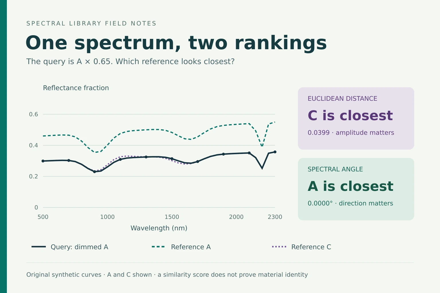
Choose “Dim the query.” The generating curve is still A, but gain is 0.65 and the ranking uses Euclidean distance. The darker look-alike C becomes the closest candidate. Switch to SAM or cosine: A returns to first place because pure positive scaling preserves direction. The experiment explains a metric disagreement without declaring either metric universally better.
Choose “Mismatch the bandpass.” The 160 nm response broadens the observed trough, while references use their centre values. Switch the reference method to the matching SRF and observe the correction. Then choose “Remove the feature.” Only 500–1,300 nm remains; A and B tie numerically because their distinguishing long-wave trough is unavailable.
Choose “Omit the true reference.” A is removed from the searchable set, although it still generated the query. The tool returns C as its closest angular match. That label is necessarily a substitute in this controlled example. Finally, “Offset + continuum” lets you explore an additive disturbance and the effect of a fitted baseline.
The ripple control is a fixed sinusoidal perturbation with an adjustable amplitude in reflectance fraction. It is deliberately deterministic, not a statistical noise distribution or a confidence interval. Download the CSV for the exact compared values or JSON for settings, rankings, warnings and provenance. The synthetic source grid is 2 nm; the sensor centres remain 50 nm apart across all FWHM settings.
Preserve ambiguity and allow an unresolved result
A closest match answers a conditional question: which supplied candidate minimizes the chosen discrepancy after these transformations? It does not establish that the physical material must occur in the library. An omitted material, weathered surface, coating, mixture or acquisition mismatch can all receive a plausible neighbour. The absent-A preset is a minimal example that requires no complicated classifier.
A runner-up gap is useful descriptive evidence, but it is not a probability of correctness. Gaps depend on the score scale and on which competing entries happen to be included. Adding another near-duplicate reference can change the margin without changing the observation. Likewise, reporting cosine 0.99 as “99% confidence” has no statistical justification.
Retain a shortlist, inspect the wavelengths that favour and contradict each candidate, and document exclusions. An operational system should be able to return “unresolved” or “outside validated coverage.” Set any acceptance threshold using representative validation data that include confusing alternatives and materials absent from the library. This tutorial intentionally supplies no universal acceptance threshold.
If the intended distinction disappears when diagnostic bands are masked or blurred, report that loss of resolving power. Neither a longer list of candidate names nor a more confident interface can supply missing information. Additional wavelength coverage, an appropriate local reference or an independent assay may be needed, depending on the claim.
Validate the identification claim you intend to make
Build the evaluation around independent physical samples and realistic acquisition conditions. Repeated scans of one specimen should not masquerade as independent evidence of material generalisation. Keep specimens, sites or acquisition sessions together when their shared properties could leak across training, threshold selection and evaluation. The spatial-split guide discusses the analogous issue for image neighbourhoods.
Test both in-library and deliberately held-out material cases. Include condition variants and near neighbours that could make the problem difficult. Evaluate the final decision, including its rejected or unresolved cases, at the level required by the application. A top-k retrieval list can be valuable for expert review even when autonomous material identification is unsupported.
Inspect stable and unstable results separately. Sensitivity tests might alter a defensible wavelength mask, the documented response uncertainty or a realistic measurement perturbation. Make those choices before examining the final test set. Report how often the candidate changes and why, without treating a deterministic perturbation sweep as a calibrated uncertainty interval.
For consequential identification, use independent evidence appropriate to the question: for example, a documented reference assay or field validation protocol. The point is to connect a spectral pattern to the material claim through observable evidence. Similarity alone supplies no chain of custody, proof of purity or chemical mass fraction.
Keep a reproducible matching record
A useful result record names the observation quantity and units; wavelength grid, response functions and quality mask; library version and sample IDs; the eligible candidate set; all conversions and preprocessing; metric formula and units; candidate scores; any rejection criterion; and the validation setting. Save the software version and numeric tolerances with those choices.
Keep the unmatched measurement alongside the processed comparison. This makes it possible to investigate whether a strong feature match concealed an amplitude or baseline disagreement. Record exclusions and absent metadata rather than dropping inconvenient entries without explanation. If a library is updated, repeat the evaluation rather than assuming the previous ranking or threshold still applies.
The practical conclusion should be narrow enough to test: these references were eligible, these candidates were most similar in these bands, and this independent evidence supports or limits the proposed identity. A carefully qualified shortlist is more useful than an unqualified material name whose provenance cannot be reconstructed.
Frequently asked questions
Does the best library match prove material identity?
No. It is the closest supplied candidate under the selected measurement, preprocessing and metric choices. Independent validation and adequate candidate coverage are needed for a material claim.
Are SAM and cosine independent checks?
No. On the same nonzero vectors, SAM is arccos of cosine similarity. Their rankings are equivalent; they present the same directional comparison on different scales.
Why do wavelength units matter if both arrays have the same length?
Array position does not establish wavelength alignment. Convert units explicitly, retain paired values, and verify the same physical bands and response functions before comparing.
Is interpolation to band centres enough?
It can differ substantially from integration over a finite band response, especially around narrow features. Use the target response functions and document any Gaussian/FWHM approximation.
Does continuum removal preserve all material information?
No. It deliberately changes the representation and removes baseline information. Its result depends on the selected wavelength window and fitted continuum.
Is this demonstration using actual USGS or ECOSTRESS spectra?
No. A, B and C are original analytic curves without physical material identities. The real libraries are linked as primary resources, but no measured spectra or third-party figures are embedded.
References and further reading
- Kokaly, R. F. et al. (2017). USGS Spectral Library Version 7. Data Series 1035. DOI: 10.3133/ds1035.
- NASA/JPL. ECOSTRESS Spectral Library, Version 1.0: collection overview and attribution.
- USGS. USGS Spectral Library Version 7 Data: data release and rights. DOI: 10.5066/F7RR1WDJ.
- NASA/JPL. JPL Spectral Library: sample preparation, grain size, ancillary information and measurement methods.
- NASA/JPL. Johns Hopkins University Spectral Library: measurement geometry and instrument documentation.
- USGS Science Data Catalog. USGS Spectral Library Version 7 Data: wavelengths, bandpasses, formats and deleted-channel values.
- NV5 Geospatial. ENVI documentation: Spectral Resampling.
- NV5 Geospatial. ENVI documentation: Spectral Angle Mapper; citing Kruse et al. (1993).
- NV5 Geospatial. ENVI documentation: Continuum Removal.
Reader feedback
Reads since 1 October 2026: at least 15 seconds with the article visible, counted once per browser per day. Reactions are anonymous and can be changed.
Loading reader feedback…
Discuss this article
Ask a technical question, challenge an assumption or share evidence from your own work.