
One spectrum, many coordinates
A hyperspectral pixel is a vector before it is a picture. Forty-eight values at forty-eight wavelengths describe one sample in this lab; an instrument may provide many more. A two-dimensional map can make those vectors easier to inspect, but it necessarily hides information. The important question is what a method chooses to preserve, and whether that matches your scientific task.
Variance, local neighbourhoods, class separation and reconstruction are different objectives. A method that produces attractive islands need not preserve spectral distances, support accurate predictions or recover the original spectrum. This guide lets you compare five actual algorithms on one small, fully disclosed synthetic dataset, with runnable source rather than decorative point clouds.
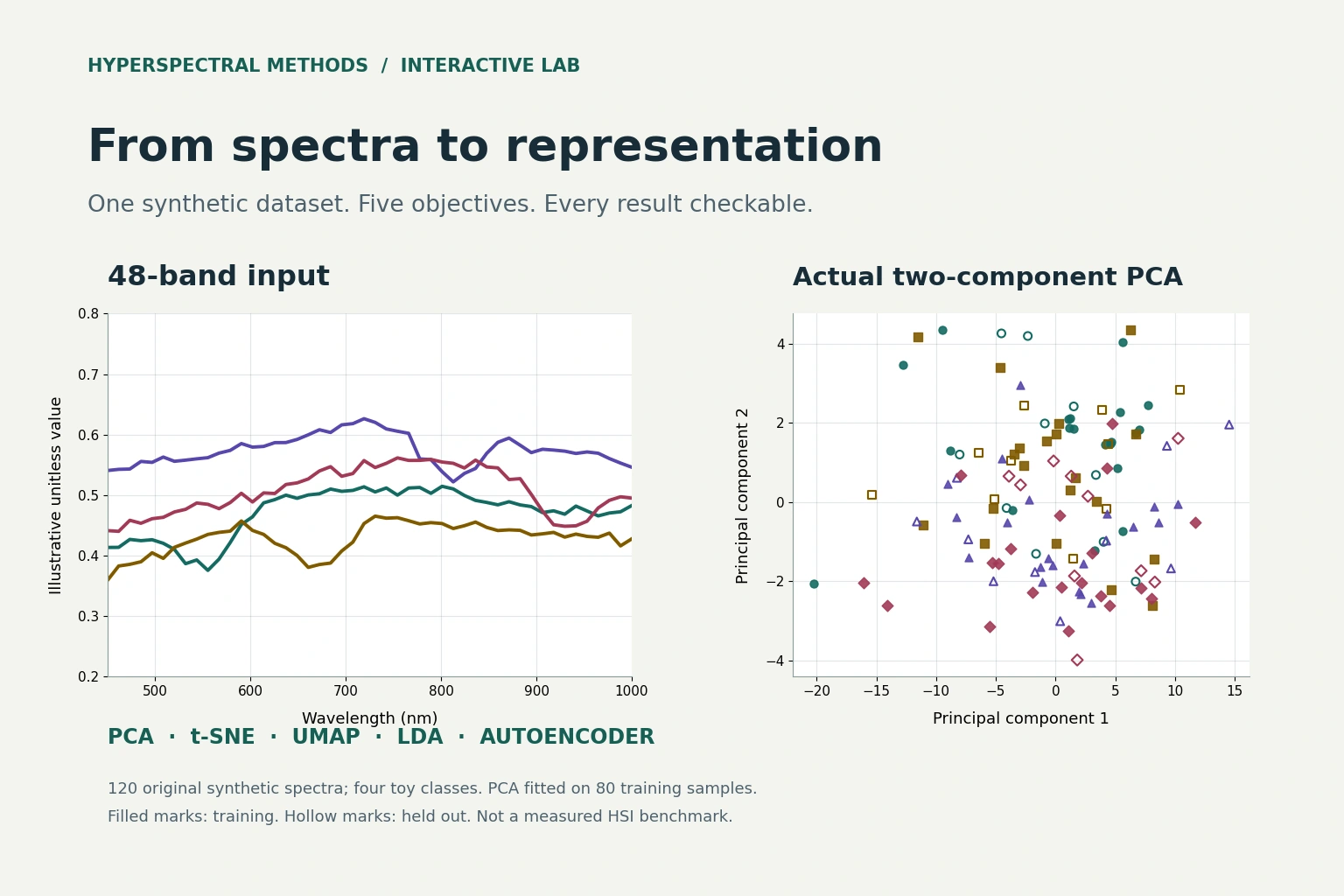
The lab is an educational experiment. Its 120 smooth spectra have four class-specific dips, brightness variation, a continuous nuisance variable and noise. They are not measured vegetation, soil, minerals or polymers. The 450–1000 nm grid provides a familiar spectral axis without claiming to simulate a particular sensor, material or acquisition process.
Separate the map from the experiment
The generator produces 30 independent spectra in each toy class. Twenty per class form a fixed training set; ten form a held-out set. The mean and optional per-band standard deviation are estimated on the 80 training rows and reused for every row. Standardising each band changes the geometry: a small-amplitude band can have as much influence as a high-amplitude one. Centre-only and unit-variance views therefore answer different questions.
PCA, Fisher LDA and the autoencoder learn from those 80 training spectra and transform the remaining 40 without refitting. LDA alone receives class labels, and only training labels. The stored t-SNE and UMAP views instead fit all 120 points together. Their hollow symbols preserve the original split identifier, but are not out-of-sample evaluations. The interface states this difference above every plot.
For a real HSI experiment, decide the unit of independence before fitting anything. Separate scenes, fields, specimens, acquisition dates or batches when your claim requires transfer across them. Fit scaling and dimensionality reduction inside the training fold. Using a test spectrum to choose a transform can already contaminate evaluation even if its label is hidden. See the spatial split guide for the broader sampling problem.
| Method | Objective | Fitting scope here | Main caution |
|---|---|---|---|
| PCA | Training variance / linear reconstruction | 80 training spectra; transform 40 | Variance can be nuisance |
| Fisher LDA | Labelled between/within-class separation | 80 training spectra and labels only | At most C−1 directions; supervised |
| t-SNE | Local similarity probabilities | All 120; stored Python runs | No global distance or holdout claim |
| UMAP | Neighbourhood graph embedding | All 120; stored Python runs | Packing is parameter-dependent |
| Autoencoder | Nonlinear reconstruction MSE | 80 training spectra; encode 40 | Low loss is not class accuracy |
PCA: what varies most?
Principal component analysis finds orthogonal linear directions ordered by variance in the fitted data. In this lab, the training covariance matrix is eigendecomposed in a browser worker. The implementation is checked against an independent scikit-learn singular-value decomposition. Component signs may flip between valid implementations, so tests compare equivalent projections rather than demanding a particular sign. [1]
The explained-variance bars refer to the training data after the selected preprocessing. Retaining two components can keep most variance while missing a small but useful class-specific dip. Here brightness is deliberately a nuisance: it can dominate variation without being the feature you want a classifier to use. High explained variance is not the same claim as high class discrimination.
Increase the retained dimensions and inspect a reconstructed spectrum. PCA compresses a centred vector into component scores, then expands it through the retained basis and restores the preprocessing scale and mean. Raw-space reconstruction error is measured over all 48 bands. When you retain more than two components, the scatter still shows only the first two, while reconstruction uses every retained component. The two displays should not be confused.
Spectral methods lab · original synthetic data
48 bands. Different questions.
Fit a projection, inspect a spectrum, and see what each objective keeps. All 120 samples are synthetic. No GPU, API key, or upload is needed.
PCA, LDA and the autoencoder fit only the 80 training spectra. t-SNE and UMAP presets fit all 120 spectra together and are exploratory.
Enable JavaScript to compute the projection. The downloadable Python code can reproduce every method.
Filled = original training split (80). Hollow = original held-out split (40). For t-SNE/UMAP, both groups participate in fitting.
- Displayed embedding
- Awaiting fit
Loading the small synthetic dataset. Controls stay disabled until it is ready.
Inspect the original spectrum
What did the method keep?
Explained variance measures training variance, not classification performance.
Read the selected spectrum as numbers
| Wavelength (nm) | Original | Reconstructed |
|---|
Read the projection as numbers
| Sample | Class | Original split | Axis 1 | Axis 2 |
|---|
Data, fitting scope and honest comparison
This fixed generator creates 30 independent spectra in each of four toy classes. A broad brightness nuisance, smooth latent variation and small noise accompany a class-specific absorption-like dip. It is not a sensor simulator or a field HSI benchmark. Samples 1–20 within each class train the learned methods; the last 10 are held out. A real HSI study needs splits by appropriate specimen, field, scene or acquisition groups.
The mean and optional per-band standard deviation always use only the 80 training spectra. PCA, Fisher LDA and the autoencoder fit those 80 rows. LDA receives only training labels. All 120 points participate in each stored t-SNE/UMAP fit; their hollow marks are original split identifiers, not out-of-sample projections. Class colours are annotations for every unsupervised method.
Neighbour overlap is the average fraction of five nearest neighbours in preprocessed 48-band space also found in the displayed 2D coordinates, over all 120 points. It is a descriptive geometry diagnostic, not accuracy, a test score or evidence of physical classes. For one retained component, axis 2 is zero. With more than two retained dimensions, the plot and overlap still use only the first two. Raw-space reconstruction MSE uses all 48 bands and all retained dimensions.
Changing settings after looking at held-out errors turns this toy holdout into a development set. Reserve a genuinely untouched test set for real conclusions. Rotation, reflection, visual cluster area and distances between t-SNE/UMAP islands are not reliable physical explanations.
t-SNE presets: scikit-learn exact solver, random initialisation, 750 iterations, automatic learning rate. UMAP presets: umap-learn, Euclidean distance, spectral initialisation, 300 epochs, one CPU thread. Seeds 7 and 29; all 36 actual outputs and version metadata ship with the source. The browser never pretends to fit these stored runs.
LDA: what separates the labels?
Linear discriminant analysis is supervised dimensionality reduction. Its directions compare the scatter of training class means with variation inside those classes. With C classes, the between-class scatter has rank at most C−1, so four classes supply at most three useful discriminant directions. A striking LDA separation partly reflects the objective using those labels; it is not independent discovery of the classes. [2]
This implementation uses regularised Fisher LDA. It solves a generalised eigenproblem with between-class scatter on one side and a ridge-stabilised within-class matrix on the other. The ridge adds the selected fraction of mean within-class diagonal variance to each diagonal element. That convention is written in the source; it is not presented as scikit-learn’s shrinkage parameter. An independent SciPy generalised eigensolver checks the resulting directions.
Try stronger regularisation and switch from two to three retained dimensions. The displayed eigenvalues are discriminant ratios, not PCA explained-variance fractions. No inverse spectrum is offered: LDA’s objective is label-related separation, not reconstruction. Test labels are not passed into the fitter, and a regression test changes every held-out label while requiring the learned directions to remain unchanged.
t-SNE: a local visual question
T-distributed stochastic neighbour embedding builds a low-dimensional arrangement whose similarity probabilities approximate similarities in the input. Its objective is useful for exploring local relationships, but interpreting large-scale distances between separated islands as physical spectral distances is unsafe. Perplexity affects the effective neighbourhood scale; it must be smaller than the number of fitted samples. [3, 4]
The lab offers perplexities 5, 20 and 40 and two random seeds. Each selection loads an actual scikit-learn exact-solver fit, using 750 iterations, random initialisation and the library’s automatic learning-rate setting. The point positions are not animated guesses, and the browser does not claim to recompute them. These small stored runs make every setting immediate on a phone; the accompanying Python command regenerates them.
Compare nearby points across settings before telling a story about a gap. Island area, orientation and distance from another island are not a calibrated account of class prevalence or physical difference. The KL objective shown is the fit’s optimisation value, not classification accuracy. This t-SNE implementation does not supply an out-of-sample transform; its full-data map is explicitly exploratory.
UMAP: the neighbourhood graph
UMAP constructs a neighbourhood-based representation and optimises a lower-dimensional embedding. The neighbourhood count changes the scale used to build the graph; min_dist influences how tightly points pack in the embedding. Larger neighbourhoods can favour broader relationships, but that is not a guarantee that global distances, densities or all topology are preserved. [5, 6]
Choose 5, 15 or 40 neighbours, min_dist 0.1 or 0.6, and seed 7 or 29. These are real umap-learn runs with Euclidean distance, spectral initialisation, 300 epochs and one CPU thread. UMAP’s Python package can transform new data, but this particular browser comparison deliberately ships full-data exploratory fits. It does not call those hollow points a validation result.
Compare a tight-packing view with a looser one. If visual islands become sharper, that may be a consequence of the selected objective and parameter setting, not new evidence that nature contains four discrete groups. The class colours are annotations. No labels enter these UMAP fits. Reproducibility metadata records library versions and seeds; reproducibility across different software or hardware environments should still be checked rather than assumed.
Autoencoders: learn to reconstruct
An autoencoder maps an input through a small latent representation and learns to reconstruct the original input. The bottleneck provides a compressed code; nonlinear layers allow a representation beyond a single linear projection. Hinton and Salakhutdinov’s work is an influential example of learning low-dimensional codes with neural networks, not a promise that every small network will outperform PCA. [7]
Here the network is deliberately tiny: 48 inputs, 12 hidden units, a two- or three-dimensional bottleneck, 12 hidden units and 48 outputs. Hidden layers use tanh; the output is linear. Full-batch Adam minimises mean squared error in the selected preprocessed space. Every run starts from seeded random weights and trains only on the 80 training spectra. The code implements actual forward propagation, backpropagation and parameter updates. [8]
Watch the training loss, then compare the original and reconstructed held-out spectrum. Lower training loss alone does not establish generalisation, and good reconstruction does not establish a useful class boundary. The plotted two-dimensional code and the decoder answer different questions, especially with a three-dimensional bottleneck. Raw-space training and held-out MSE are reported separately from the scaled training loss.
The 100, 250 and 500 epoch choices are bounded teaching budgets. Training runs in a Web Worker; Cancel terminates it and leaves any previous result intact. A 20-second device limit prevents a long-running fit on a slower phone. There is no GPU dependency, paid API, external model call or hidden pretraining.
Measure the right loss
The five-neighbour overlap is a deliberately simple geometric diagnostic. For each of all 120 points, find its five nearest neighbours in the preprocessed 48-band space and in the displayed two-dimensional coordinates. Count how many identities occur in both sets, divide by five, then average across points. The downloadable result contains the actual coordinates behind the diagnostic.
This value is not a held-out prediction metric, does not use labels and is not called trustworthiness. It ignores the rank of a misplaced neighbour and depends on preprocessing, neighbourhood size and the displayed dimensions. A high value can preserve brightness nuisance very well. A low value can accompany an LDA map that deliberately emphasises class separation instead of the original Euclidean geometry.
Reconstruction MSE compares original and reconstructed values in the original synthetic band scale, averaged across samples and bands. It is available only for PCA and the autoencoder in this lab. It remains a teaching diagnostic: if you repeatedly select settings using the displayed held-out result, that set has become part of development. A final scientific comparison requires independent evaluation, appropriate uncertainty and a task-relevant outcome.
Make the code a checkable claim
The browser uses dependency-free ES modules for the local algorithms and a small JSON bundle for verified t-SNE/UMAP outputs. The downloadable source contains the generator, all algorithm code, pinned Python requirements, a notebook, tests and a manifest. Run the Python reproduction command to rebuild the data, numerical fixtures and all 36 stored embeddings from scratch on a CPU.
Tests compare PCA with scikit-learn SVD, regularised LDA with SciPy and the trained autoencoder with an independent NumPy implementation. A finite-difference test checks every parameter gradient on a tiny network. Other tests check split isolation, parameter rejection, deterministic outputs, complete presets and finite plot geometry. These checks support the implementation, not external performance claims.
The practical sequence is to choose the scientific task first, choose a transform whose objective makes sense for it, fit only on permissible training data and evaluate the downstream claim independently. Use these maps to ask better questions about spectra. Do not let a pleasing arrangement of coloured points answer questions the experiment never tested.
Frequently asked questions
Which dimensionality reduction method is best for HSI?
It depends on the task. PCA targets variance, LDA uses training labels, t-SNE and UMAP explore neighbourhood structure, and an autoencoder learns reconstruction. Evaluate the downstream task on appropriately independent data.
Does explained variance measure classification accuracy?
No. Large spectral variance may reflect illumination or another nuisance. A discriminative feature can occupy a low-variance direction.
Why can four classes produce only three LDA directions?
The between-class scatter is built from four class means around a common mean and has rank at most C−1. This lab therefore limits LDA to three directions.
Are t-SNE and UMAP fitted live in this browser?
No. Their controls select 36 genuine, seeded Python runs included in the source. PCA, LDA and the small autoencoder fit locally in a browser worker.
Are the hollow t-SNE and UMAP points held-out predictions?
No. They identify the original split, but every point participated in those exploratory fits. The interface labels that scope explicitly.
Can I run all the code without a GPU or paid API?
Yes. The static browser lab needs no external runtime dependency. The Python reproduction and notebook use the supplied CPU dependencies to regenerate all method outputs.
References and further reading
- scikit-learn. PCA API: centring, components, explained variance and inverse transform.
- scikit-learn. Linear and Quadratic Discriminant Analysis: dimensionality reduction and mathematical formulation.
- van der Maaten, L. & Hinton, G. (2008). Visualizing Data using t-SNE. JMLR 9, 2579–2605.
- scikit-learn. TSNE API: perplexity, initialisation, learning rate and iteration controls.
- McInnes, L., Healy, J. & Melville, J. (2018). UMAP: Uniform Manifold Approximation and Projection for Dimension Reduction.
- UMAP documentation. Basic UMAP Parameters and reproducibility guidance.
- Hinton, G. E. & Salakhutdinov, R. R. (2006). Reducing the dimensionality of data with neural networks. Science 313, 504–507.
- Kingma, D. P. & Ba, J. (2015). Adam: A Method for Stochastic Optimization. ICLR.
Reader feedback
Reads since 1 October 2026: at least 15 seconds with the article visible, counted once per browser per day. Reactions are anonymous and can be changed.
Loading reader feedback…
Discuss this article
Ask a technical question, challenge an assumption or share evidence from your own work.