
Define the output before choosing a tile size
An out-of-core pipeline should produce the intended result while keeping its working arrays bounded. Splitting a cube into rectangles is the easy part. The difficult part is preserving context, edge behaviour and output coordinates when those rectangles are processed independently.
This guide builds and tests a small finite-context example. It compares complete output logits, deliberately introduces seams, checks stride alignment and writes results incrementally. The example is synthetic, CPU-only and implemented in NumPy. Its coefficients are fixed teaching values, not a trained HSI classifier or a benchmark of any published model.
The hardware and software guide already covers cube-size arithmetic and general memory budgets. Here the question is narrower: how do you change execution order without silently changing the calculation? The preprocessing guide explains how to establish the spectral representation first.
Bound the working set through the entire pipeline
Begin with a reader that accepts a spatial window, a transform that operates on that window and a writer that accepts an output window. Keep the band axis intact when the calculation mixes all bands. Convert the data type and standardise inside the window, rather than converting the complete cube before the tile loop.
A file-backed input does not make subsequent expressions allocation-free. NumPy memmap exposes file-backed array access, but arithmetic, dtype conversion and downstream work can still allocate arrays. Touched mapped pages also occupy physical memory. The bounded quantity in this example is the model’s tile-sized working data, not a promise that total process RSS stays constant as a file grows. [4]
Do not append every tile prediction to a Python list and concatenate it at the end. Write the retained core directly into a file-backed output, or into a writer that commits windows. Count live inputs, temporary arrays, activations, queued work and outputs together. A large worker or prefetch queue can undo the benefit of a small tile.
Sources: [4]
| Check | Eager reference | Tiled path |
|---|---|---|
| Input representation | H × W × B float32 | Same representation per read window |
| Spatial context | Complete domain | Sufficient halo; core retained |
| True image edges | Available-neighbour mean per layer | Same edge rule |
| Output grid | Global stride-two origin | Aligned read and core origins |
| Output storage | Mapped result after full computation | Incremental mapped core writes |
Work out which outputs depend on which inputs
The supplied model standardises each spectrum with fixed per-band constants, projects it to four channels, applies two 5 × 5 neighbourhood means with tanh nonlinearities, and projects to three logits. It then samples every second spatial position. Before that final sampling, each output depends only on inputs within four pixels in each spatial direction: two radius-two operations compose to radius four.
For a simple chain of convolution or pooling layers, track receptive-field size and sampling jump separately. Starting with size r = 1 and jump j = 1, a layer with kernel k, dilation d and stride s gives r_new = r + (k − 1) × d × j, then j_new = j × s. Padding also changes the output-grid offset. Even kernels, asymmetric padding, branching, resizing and decoder paths require additional bookkeeping; a single radius is not a complete specification. PyTorch’s convolution documentation exposes the relevant shape parameters. [5]
A sufficient halo follows from that dependency calculation. It is not a percentage selected because the stitched image looks plausible. The harness uses a conservative four-pixel halo. Its final stride-two sampling and alignment can make some smaller nominal halos sufficient for particular retained pixels; that is not a general minimal-halo claim.
Sources: [5]
Tile seams · synthetic CPU fixture · finite context
How much of the border can you keep?
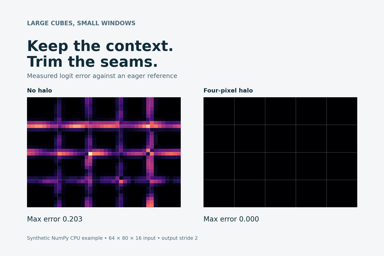
Choose the input halo around each 16 × 16 core. The model sees two radius-two spatial filters and samples every second pixel. The right map shows the largest absolute logit error across three outputs at each location, compared with one eager run.
Exactly zero 10⁻⁶ or smaller nonzero 10⁻² 1 or larger. Fixed logarithmic scale for nonzero errors; grid lines show core boundaries.
Static result: no halo gives max error 0.2032; aligned halo 4 gives zero. Interactive controls load when JavaScript is available.
The browser displays saved results from the tested NumPy script, rather than running a neural network. Input: 64 × 80 × 16, float32. Output: 32 × 40 × 3. No sensor data or model-accuracy claim. Test criterion: |difference| ≤ 2 × 10⁻⁶ + 10⁻⁵ × |reference|.
Download Python code and tests · Download the executed notebook · Download the measured CPU report
Read the halo and write only the core
Partition the output into non-overlapping core regions. For each core, expand the input read by the required halo, clip that read to the real image extent, run the transform and trim away predictions belonging to the overlap. Write only the retained core. This makes output ownership unambiguous: every output sample is written exactly once.
For a 96 × 96 core and halo four, an interior read is 104 × 104. Its pixel-area overhead is 104² / 96², about 17.4%, before storage blocks and alignment are considered. Edge windows contain fewer extra pixels. Larger cores usually reduce this repeated work but increase the working set. Choose a core after both correctness and peak-memory checks.
The implementation exposes separate reader and writer callbacks. Its tests record output-write counts, require every count to equal one and reject an incompatible core/stride combination. Those checks catch missing strips and accidental double writes that may be hard to spot on a colour map.
Preserve the real image edge rule
The synthetic model averages only available in-domain neighbours at each spatial layer. At a corner, a radius-two mean therefore has fewer contributing values than at an interior pixel. The denominator changes with the available neighbourhood. A constant input remains constant all the way to the real border.
An internal tile boundary is artificial. Its local edge rule can influence nearby intermediate values, but a sufficient halo keeps that influence outside the retained core. At the real scene boundary, the cropped tile and eager model see the same domain boundary and use the same per-layer rule. The harness tests both conditions.
Changing the example to zero padding, reflection or another policy requires matching that policy in the reference and tiled path. Padding the original cube once is not automatically equivalent to applying padding inside every layer. No-data is a separate contract: this example rejects non-finite input and does not claim to implement a sensor mask, missing-spectrum interpolation or masked-network inference.
Keep the output sampling grid anchored to the scene
A correct halo can still produce the wrong coordinates. With output stride two, an eager run keeps global rows 0, 2, 4 and so on. A tile whose read begins at row 11 would naturally keep global rows 11, 13, 15 if its local output is sampled from zero. Cropping cannot relabel those measurements into the correct global positions.
The tested planner makes each read origin a multiple of the output stride by rounding its top and left bounds outward. Core starts are also stride-aligned. The trim offsets are then exact integers in output coordinates, and odd-sized final cores are handled with ceiling division. Read origins can expand by up to stride minus one additional pixels beyond the requested halo.
The viewer’s deliberate failure mode removes that alignment and uses a naive local crop. Even a five-pixel halo then fails the logit comparison. For a real encoder-decoder, propagate both output stride and offset through the complete architecture and test its actual output geometry. The demonstration’s final decimator is intentionally simpler.
Compare logits before comparing class labels
Argmax can hide changed predictions when the winning class stays the same. Save an eager reference for a manageable scene, compare complete logits and report the largest absolute difference, mean absolute difference and fraction of changed labels. Inspect errors separately near core joins and at true image borders.
This harness tests |tiled − reference| ≤ 2 × 10⁻⁶ + 10⁻⁵ × |reference|, using float32 throughout. Those tolerances are declared for this fixture, not universal acceptance thresholds. Exact zero happened on the measured runs. Other implementations, shapes and hardware may change floating-point reduction order; PyTorch explicitly cautions against assuming bitwise identity across execution arrangements. [7]
For the 64 × 80 × 16 viewer fixture, no halo gives a maximum logit difference of 0.203161 and changes 2.58% of labels. Halo two still fails. With halo four and an aligned grid, all compared logits match exactly in this run. The intentionally misaligned halo-five case changes 6.80% of labels. These are equivalence results on synthetic values, not classification accuracy.
Sources: [7]
A small measured CPU comparison
On 2 October 2026, the supplied harness ran in a Linux x86_64 container reporting an Intel Xeon Platinum 8573C, using Python 3.12.14 and NumPy 2.3.5. Numerical-library thread limits were set to one. The input was a coordinate-defined 768 × 1024 × 32 float32 cube with 96 MiB of elements. There was no GPU execution.
Three fresh-process runs per method produced median wall times of 0.302 s eager and 0.306 s tiled. Measured process high-water RSS was approximately 406.5 MiB eager and 123.6 MiB tiled. The timing difference is too small and environment-specific to support a general speed claim. The useful observation is that this implementation retained equivalent outputs with a substantially smaller measured working footprint.
The tiled path processed 88 cores of up to 96 × 96, with halo four and output stride two. Its largest input view was 104 × 104 × 32, or about 1.32 MiB of elements. Total requested pixel area was 1.157 times the scene area. That figure counts the harness’s windows; it does not measure bytes fetched by a compressed reader or a storage device.
The timing includes mapped-output allocation, input access or copying, calculation, writes and output flush. It excludes interpreter imports and fixture construction. The file had just been generated and caches were not evicted, so this is not a cold-storage benchmark. RSS comes from Linux /proc/self/status VmHWM for each fresh process and includes interpreter, libraries and resident mapped pages. The eager implementation intentionally owns a full input copy before its full-scene transforms. Different eager implementations can have different peaks.
Connect the contract to an HSI reader
Rasterio reads and writes rectangular windows, but it fills requests through the file’s storage blocks. A small requested window can trigger a much larger underlying read. Inspect block_shapes and access patterns; coordinate block alignment with model-grid alignment rather than assuming they are identical. Its window_transform helper describes a cropped window’s spatial transform. [1]
Rasterio commonly supplies arrays in band, row, column order, while this harness expects row, column, band. Make that conversion explicit at the reader boundary. Retain scale factors, wavelength order and masks in the surrounding contract. For same-resolution outputs, preserve the intended geospatial grid. For strided output, derive the affine transform from the actual retained sample centres and footprint convention; copying the input transform or only changing the dimensions can misregister the result.
Spectral Python opens a SpyFile with metadata first and reads requested values on demand. Its load method materialises a float32, row-column-band ImageArray; open_memmap is the file-backed alternative. Choose the access route deliberately rather than calling load before a supposedly out-of-core loop. Repeated ordinary SpyFile reads are not cached by that object. [3]
The downloadable core harness runs with NumPy alone. Rasterio and Spectral Python are integration options discussed from their documentation; they were not installed or executed for the measured benchmark.
Use Dask overlap with the same boundary contract
Dask map_overlap expands chunks with neighbouring data, applies a function and normally trims the overlap. depth controls overlap by axis, boundary controls the outside-domain policy and trim determines whether Dask removes the expanded borders. It can rechunk when overlap exceeds a chunk dimension; inspect that behaviour and the resulting task graph. [2]
For a shape-preserving local transform on an H × W × B array, a starting design is depth={0:4, 1:4, 2:0}, the whole required spectral axis in each chunk, and an explicitly chosen boundary policy. For this available-neighbour model, boundary="none" allows its own true-edge handling. Avoid giving Dask and the function contradictory padding or trimming responsibilities.
The supplied final output decimation changes spatial shape. Do not copy the shape-preserving recipe unchanged: chunk output sizes, offsets and stride phase must be worked through. A useful first Dask validation is a dense shape-preserving version of the operator, followed by a separate globally anchored selection. Bound concurrent tasks and store the result incrementally; collecting the full result can reintroduce the allocation you meant to avoid. No Dask equivalence or performance run is claimed here.
Sources: [2]
Identify operations a finite halo cannot reproduce
A finite halo cannot generally reproduce global attention, whole-scene spatial normalization or unrestricted recurrent and state-space context. With global attention, excluded keys can change both the weighted values and the normalization. With a scan-based model, resetting state at a tile boundary changes the history. A larger local window may reduce the discrepancy without proving equivalence.
Some global operations have an exact streaming formulation. A mean can be accumulated in a first pass and applied with fixed statistics in a second. A directional recurrence may permit a carefully ordered traversal with carried state. Other architectures need different algorithms, model changes or an explicitly approximate tiled mode. Name that approximation and measure its effect rather than describing finite overlap as universally exact.
Per-tile standardisation also changes the function unless the reference is defined that way. Keep learned preprocessing fixed from its authorised training fit, as explained in the spatial-split guide. Averaging overlapping logits can reduce visible seams, but blending cannot reconstruct dependencies the tile never received.
Keep inference state and gradient mode explicit
For PyTorch inference, put the model in evaluation mode and use an appropriate no-gradient context. torch.inference_mode() does not automatically call model.eval(); dropout and batch-normalisation behaviour still depend on model mode. [6] Those settings help establish a stable reference, but they do not convert global operations into local ones.
Check which axes each normalisation layer reduces over. A layer that still uses the current tile’s spatial statistics can change when the tile changes. Preserve dtype and preprocessing, account for device transfers and measure actual tensor and process memory in that implementation. The NumPy CPU figures above predict neither GPU peak memory nor throughput, and they do not validate training-time tiling.
Sources: [6]
Make the equivalence test part of the pipeline
The downloadable test suite covers partition-invariant synthetic values, sufficient and insufficient halos, real image edges, odd shapes, output strides one through three, a single-pixel image, bounded read windows, exactly-once writes, non-finite rejection and mapped-file round trips. It includes deliberate seam and phase failures so a broken checker cannot pass silently.
Re-run these checks on a small representative real input before a production scene: fix the reader, metadata, model state and output-grid contract; compare several core sizes and origins; include borders and no-data cases; then measure peak memory and timing under the actual scheduler. Keep the full source, parameters and measured report with the result.
The practical stopping condition is an output you can account for and a working set that fits its budget. A stitched map that looks smooth is useful for inspection, but the numerical contract is what makes tiled processing trustworthy.
Frequently asked questions
Does memory mapping mean the calculation uses no RAM?
No. Mapped pages become resident and arithmetic, conversions, activations and output buffers may allocate memory. Keep the whole pipeline bounded and measure process peaks.
Can a halo make every neural network exactly tileable?
No. Finite local context can be handled this way, but global attention, some normalisation and unrestricted state need a different exact algorithm or an explicitly tested approximation.
Why compare logits if the labels are identical?
Argmax hides differences that do not change the winning class. Logit checks reveal numerical changes before they appear as label seams.
Is a four-pixel halo always enough?
Only for the finite dependency structure tested here, with its edge and output-grid rules. Derive context and offsets for the complete operation you actually run.
Why can a correct halo still give a different output?
The output sampling grid must stay aligned to the scene. A tile-local stride can select different pixels even when enough spatial context is available.
Do the reported CPU measurements predict GPU performance?
No. They describe the supplied NumPy implementation and tested container. Measure memory, throughput and numerical agreement on the actual implementation and device.
References and further reading
Reader feedback
Reads since 1 October 2026: at least 15 seconds with the article visible, counted once per browser per day. Reactions are anonymous and can be changed.
Loading reader feedback…
Discuss this article
Ask a technical question, challenge an assumption or share evidence from your own work.