
What hyperspectral imaging measures
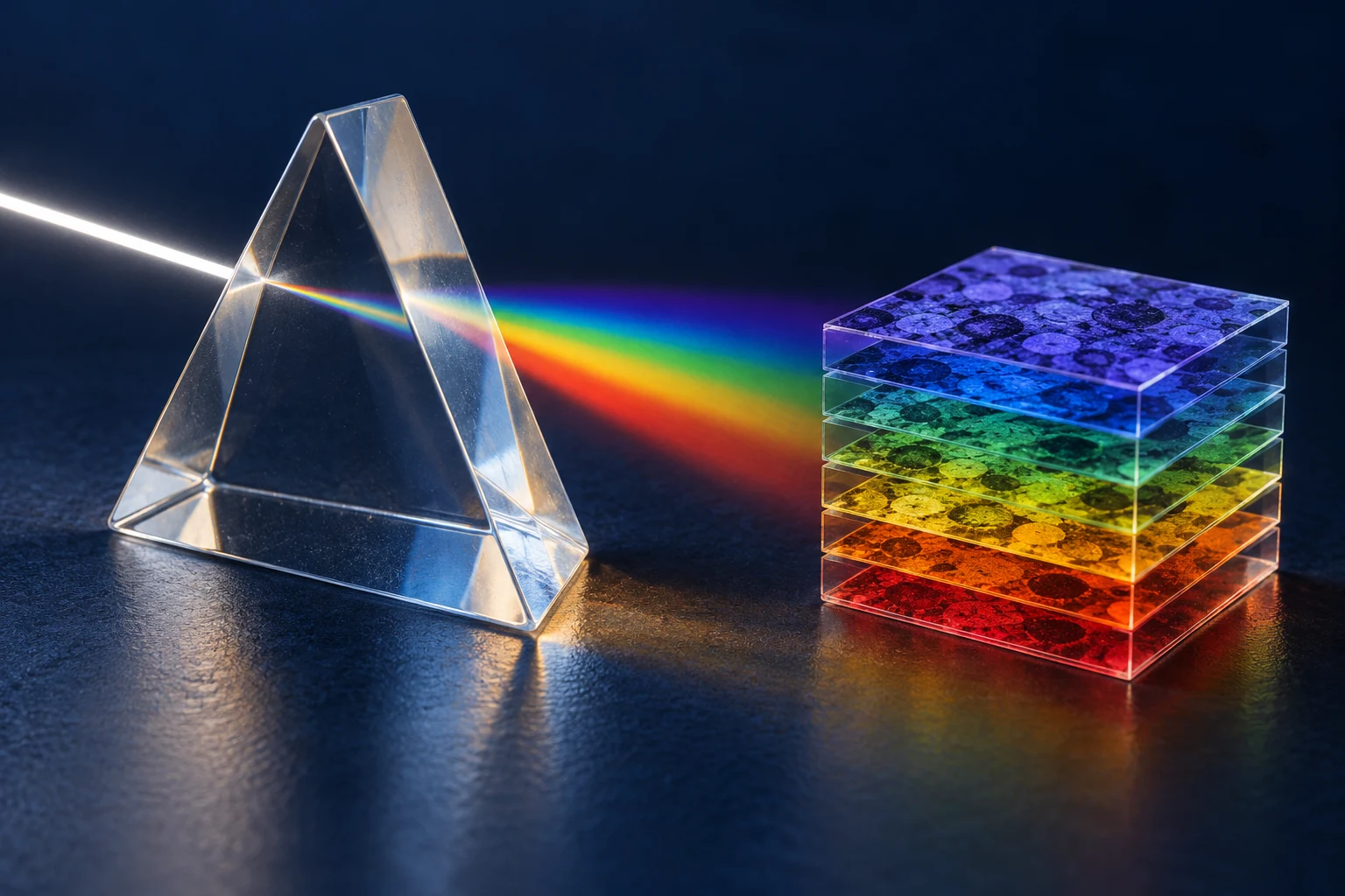
Hyperspectral imaging, often shortened to HSI, measures how light varies with wavelength at many positions in a scene. A conventional colour photograph stores three broad channels. An imaging spectrometer instead records many comparatively narrow bands, usually arranged next to one another across a defined wavelength range. Each image position therefore has a sampled spectrum as well as a location. NASA describes this combination as imaging spectroscopy. 1
The useful question is what those measurements can reveal. An absorption feature may help distinguish a mineral, changes in a plant spectrum may indicate a physiological difference, or spatial variation may locate a material within a mixed object. The camera does not attach a chemical name to each pixel. Interpretation requires a relevant spectral feature, an appropriate physical or statistical method, and evidence that the method works for the scene being measured.
This tutorial focuses on reflected light. Hyperspectral instruments can also measure emitted radiation, including thermal emission, but the calibration and interpretation differ. Start by identifying the physical quantity in the dataset rather than assuming every cube contains reflectance. NASA's HyTES is an example of a thermal imaging spectrometer. 9
Read a cube in three directions
Represent a cube as C(x, y, λ), where x and y identify spatial positions and λ denotes wavelength. Fixing λ produces a band image. Fixing x and y produces a spectrum. Selecting a region and averaging its pixels produces a regional spectrum, which can reduce random noise but can also conceal small features or mix different materials. 10
The word cube describes three indexed dimensions, not equal dimensions. A synthetic dataset with 640 columns, 480 rows and 200 bands contains 61,440,000 values. At two bytes per value it needs 122,880,000 bytes, about 122.9 MB or 117.2 MiB, before headers, masks and additional products. This explains why even modest images can require substantial memory.
A spectrum plotted as a smooth line still contains discrete, finite-bandwidth measurements. Joining the points makes a figure readable; it does not create new observations between them. Preserve the wavelength vector, the units and any invalid-band mask when exporting or reshaping a cube.
Sources: [10]
| Characteristic | Multispectral imaging | Hyperspectral imaging |
|---|---|---|
| Spectral measurement | A selected set of wavelength bands | Many narrow, commonly contiguous bands |
| Typical use | Monitor known, validated spectral contrasts | Explore spectral structure and map materials |
| Data per spatial sample | Usually fewer values | Usually more values |
| Spatial resolution | Determined by the complete imaging system | Determined by the complete imaging system |
| Main selection question | Are the selected bands sufficient? | Does the additional spectrum improve the decision? |
Separate wavelength range, sampling and resolution
Wavelength range states which part of the spectrum is covered. Spectral sampling states the spacing between recorded band centres. Spectral resolution describes the instrument's ability to distinguish nearby spectral structure and is commonly characterised by a response width, often its full width at half maximum, or FWHM. A 2 nm sampling interval and a 10 nm response width are different specifications. Recording more closely spaced bands does not automatically make the optical response narrower. 2
Spatial sampling describes the distance represented by neighbouring image samples, in millimetres on a laboratory object or metres on the ground. Spatial resolution also depends on optics, focus and motion. If two objects occupy one pixel, their contributions can be mixed even when the spectrum is finely sampled. Better spectral information cannot recover spatial detail that the acquisition did not resolve.
Published instrument examples show why the distinctions matter. NASA lists AVIRIS as providing 224 contiguous spectral channels spanning approximately 380 to 2510 nm. USGS separately reports spectral sampling and spectral resolution for the point spectrometer used in a HySpex calibration dataset. These numbers describe specific instruments and configurations, not a universal HSI specification. 6 7
Explore an illustrative spectrum
Synthetic reflectance at fixed wavelengths. This is a teaching curve, not a measured material signature.
Distinguish counts, radiance and reflectance
Raw digital counts depend on the detector, exposure, gain, illumination and sample. Radiometric calibration converts counts into a physical quantity such as spectral radiance, commonly expressed in W m⁻² sr⁻¹ nm⁻¹. Radiance describes light travelling towards the sensor. Reflectance relates reflected to incident radiation; reported reflectance factors also depend on measurement geometry. A brighter radiance value does not necessarily mean a more reflective material. 4
For a stable laboratory arrangement, a common reference-based approximation is R̂(λ) = [(S(λ) − D(λ))/(W(λ) − D(λ))] Rref(λ). S is the sample signal, D the dark signal, W the reference signal and Rref the certified reference reflectance. With illustrative counts S = 550, D = 50 and W = 1050, and Rref = 0.99, the estimate is 0.495. The calculation applies wavelength by wavelength and assumes a linear, unsaturated response and suitably matched measurement conditions.
This ratio cannot repair saturation, a changed lamp, a dirty reference or unequal geometry. An airborne or satellite measurement also includes atmospheric effects, so deriving surface reflectance needs an appropriate atmospheric correction. The reference calculation is useful precisely because its assumptions are explicit.
Compare HSI with multispectral imaging
Multispectral imaging records a selected set of bands, often broader and more widely separated than HSI bands. It can answer a well-defined question efficiently when the necessary spectral regions are already known. Hyperspectral imaging provides a richer sampled spectrum that can help explore which regions contain useful differences. Band count alone is an incomplete definition: coverage, response width and placement all matter. 3
The tradeoff is task dependent. A narrow absorption can be diluted when a sensor averages over a wide band. Conversely, hundreds of bands add little value if a decision only needs a few stable measurements. A bespoke multispectral system may therefore be suitable after an HSI study has established and validated a small band set.
Avoid equating spectral richness with sharper images. NASA's description of Landsat's Operational Land Imager separates its 15 m panchromatic and 30 m multispectral sampling. Spectral and spatial specifications should be compared independently, alongside coverage, noise, revisit or acquisition time and processing requirements. 8
Try an illustrative band-width calculation
The Python example defines a smooth synthetic reflectance curve with two absorption features and averages it through ideal rectangular bands. It needs Python 3 and only the standard library. No measurements, downloads or fitted model are involved. Run it as a script and compare the values for 5, 20 and 50 nm widths.
The band measurement is approximated by Rband = (1/b) ∫ R(λ) dλ over a band of width b. The code evaluates this integral with midpoint sampling. Increasing the width raises the measured reflectance at the centre of a narrow absorption because the band includes brighter neighbouring wavelengths. Real sensors have response functions that are not necessarily rectangular, so this is a teaching example rather than a simulated camera specification.
Use the same idea interactively by changing band width while keeping the underlying spectrum fixed. The graph should show the fine synthetic curve and the averaged band values. Label both axes and identify the data as synthetic so readers can see which change comes from the measurement and which comes from the material.
A practical workflow for your first cube
Begin with the metadata. Confirm the array order, wavelength units, data units, calibration level, exposure and acquisition geometry. Then inspect a few individual bands, spectra from several locations, and masks for missing or saturated data. A colour composite is useful for orientation, but three displayed bands cannot show the quality of the entire spectrum.
When comparing a spectrum with a library, account for the camera's wavelength range and response. USGS maintains documented reflectance spectra for minerals, vegetation, mixtures and manufactured materials. These are valuable references, but a library spectrum is not a guarantee that the same material will be uniquely identifiable in an arbitrary image. Grain size, mixtures, surface condition and observation geometry can change the measured result. 5
Finally, state the intended output and the evidence needed to check it. A material map needs independently checked locations; a concentration estimate needs reliable reference measurements. Record processing steps and retain the original data so an apparent spectral feature can be traced back to the measurement.
- Check saturation before interpreting an absorption or a flat spectrum.
- Compare wavelength range and band response before comparing instruments.
- Keep raw measurements, calibration references and processing metadata together.
Run the example
Prerequisite: Python 3. Examples use synthetic inputs to explain the calculation. Save the snippet as example.py and run python3 example.py.
from math import exp

def reflectance(wavelength):
    return (0.60
            - 0.25 * exp(-0.5 * ((wavelength - 700) / 8) ** 2)
            - 0.12 * exp(-0.5 * ((wavelength - 760) / 14) ** 2))

def band_mean(centre, width, points=10000):
    step = width / points
    left = centre - width / 2
    return sum(reflectance(left + (i + 0.5) * step)
               for i in range(points)) / points

for width in (5, 20, 50):
    print(f'{width:d} nm: R700={band_mean(700, width):.3f}, '
          f'R760={band_mean(760, width):.3f}')
Verified output
5 nm: R700=0.354, R760=0.481
20 nm: R700=0.402, R760=0.489
50 nm: R700=0.499, R760=0.522
Frequently asked questions
How many bands make an image hyperspectral?
There is no useful universal band-count threshold. Narrow, closely spaced measurements and their wavelength coverage matter more than the label.
Is every hyperspectral cube a reflectance cube?
No. A cube may contain raw counts, calibrated radiance or a derived reflectance product. Check its metadata and units.
Does finer spectral sampling mean better resolution?
Not automatically. Sampling is the spacing between band centres; resolution concerns the instrument's response to nearby spectral features.
Can I average all pixels before analysis?
Only if the average answers your question. Averaging can reduce random noise while concealing variation or mixing distinct materials.
Why can two measurements of a material differ?
Illumination, geometry, calibration, mixtures and surface condition can change the measured spectrum. Compare conditions before attributing a difference to chemistry.
Should I choose HSI over multispectral imaging?
Choose based on the required information and validated performance. More bands help when they preserve spectral distinctions relevant to the decision.
References and further reading
- NASA JPL: Imaging spectroscopy
- NIST: Spectral resolution
- Specim: Hyperspectral and multispectral cameras
- Resonon: Raw, radiance and reflectance data
- USGS: High resolution spectral library
- USGS: Calibrated HySpex measurements at Cripple Creek
- NASA JPL: AVIRIS instrument
- NASA: Landsat Operational Land Imager
- NASA JPL: Hyperspectral Thermal Emission Spectrometer
- HySpex: Hyperspectral cameras and imagery