
Plan the measurement before choosing a camera
A hyperspectral cube needs two spatial dimensions and a wavelength dimension. Acquisition systems assemble those dimensions in different ways, which changes how they respond to motion, weak light and changing illumination. Begin with the scene: is it stationary, moving predictably on a conveyor, or changing while you observe it? Then define the required spatial detail, wavelength range and acceptable acquisition time.
There is no capture architecture that is best in every situation. A laboratory stage can provide controlled motion and lighting. An aircraft provides forward motion but requires navigation and geometric processing. A rapidly changing scene puts pressure on methods that capture locations or wavelengths at different times. The relevant comparison is the complete measurement, including optics, mechanics, references and processing.
Write down the intended output before purchase or data collection: a material map, an average spectrum or a calibrated concentration estimate. This makes it possible to evaluate whether acquisition artefacts could change the decision rather than judging a camera solely by band count.
Pushbroom: record a line and move through the scene
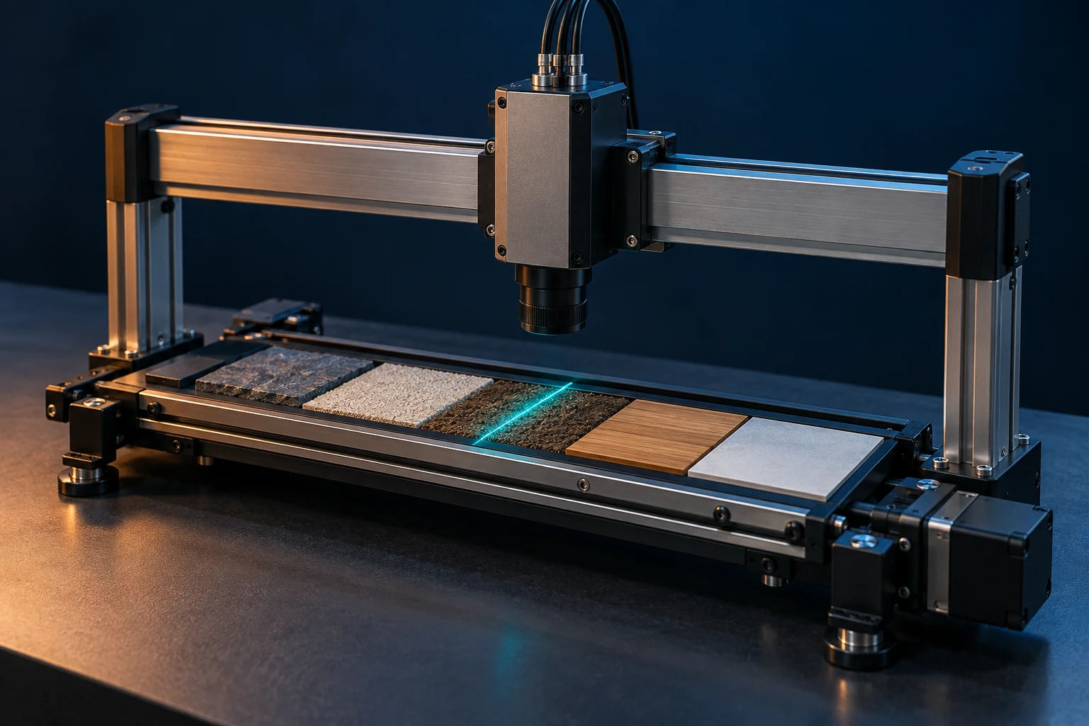
A pushbroom, or line-scan, imaging spectrometer measures one spatial line with spectral information for positions along that line. Relative motion supplies the second spatial dimension. Resonon's benchtop documentation describes moving a sample on a translation stage to construct the image. A conveyor, translating camera or airborne platform can provide the same necessary relative motion in other systems. 1
The line acquisition must be coordinated with motion. Under constant translational speed v and line rate f, the distance between lines is Δy = v/f. At an illustrative 100 mm/s and 200 lines/s, it is 0.5 mm. Exposure time matters separately: movement during a 2 ms exposure is v t = 0.2 mm. Neither number alone establishes spatial resolution, because focus, slit width and the optical response also contribute.
Pushbroom systems fit predictable continuous movement well, but speed variation, vibration and changing illumination can distort the assembled image. NASA identifies AVIRIS-NG as a pushbroom instrument. Its published 380–2510 nm coverage and 5 nm spectral sampling illustrate one airborne implementation rather than the capability of every line-scan camera. 3 10

| Architecture | Acquisition unit | How the cube is assembled | Main practical concern |
|---|---|---|---|
| Pushbroom | One spatial line with spectral information | Relative motion supplies the second spatial dimension | Motion coordination and variation between lines |
| Whiskbroom | Sequential spatial positions | Across-track scan plus motion or a second scan | Scan mechanics, dwell time and positional timing |
| Snapshot | Scene information in one exposure or snapshot measurement | Optical mapping or encoding and reconstruction | Allocation of detector information and spectral fidelity |
| Tunable filter | One selected band image | A sequence of wavelength images | Change or movement between wavelength acquisitions |
Whiskbroom: scan positions across a line
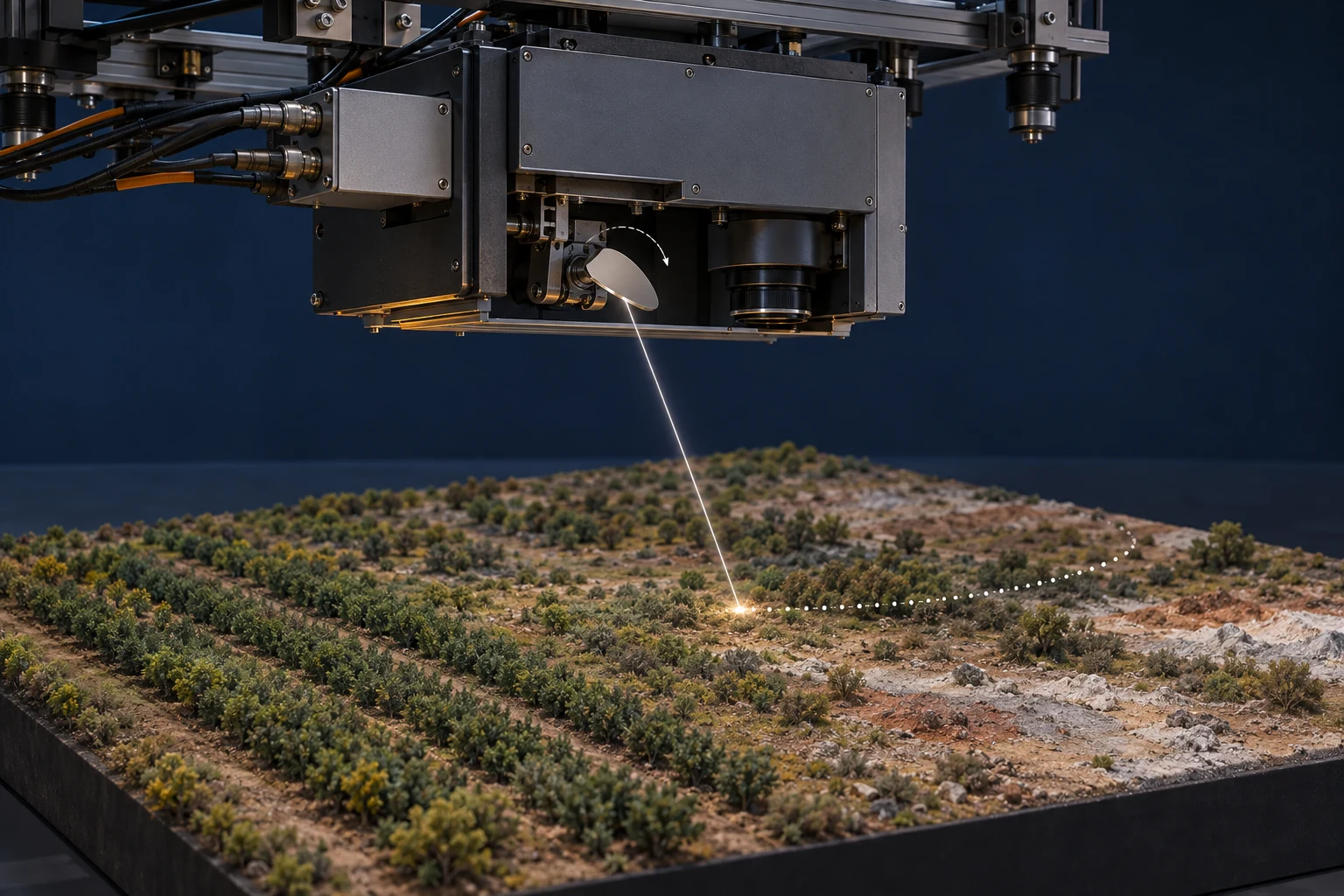
A whiskbroom system scans spatial positions across the scene, typically using a moving optical element, while platform motion or a second scan builds the other spatial dimension. The classic AVIRIS user's guide describes that instrument as a nadir-viewing whiskbroom scanner. It should not be confused with the pushbroom architecture of AVIRIS-NG. 2
Because positions are acquired sequentially, scan timing and platform position are part of the geometric measurement. A changing scene can therefore appear inconsistent across a sweep. The dwell time available at each location, scan mechanics and calibration strategy matter alongside wavelength specifications.
The architecture remains a useful concept even when evaluating a laboratory scanner. Ask which scene locations are measured simultaneously and which are measured later. That timing determines whether object movement, a flickering light or a transient event could be mistaken for a spatial difference.
Sources: [2]
Estimate line-scan acquisition time
Synthetic pushbroom acquisition: 1000 lines, constant line rate, excluding start-up, reference capture and transfer overhead.
Snapshot: acquire the scene without a spatial scan
Snapshot hyperspectral systems acquire spatial and spectral information within a single exposure or snapshot measurement, depending on the design. This reduces the need to assemble a changing scene from successive scan lines or successive wavelength images. It does not mean every detector pixel directly measures an independent, full-resolution spectrum.
Some systems redistribute image regions optically so that spectra can occupy different detector locations. Gao and colleagues reported an image mapping spectrometer for hyperspectral microscopy. Other systems encode spectral information and reconstruct a cube computationally. Deng and colleagues demonstrated a snapshot method using spectral-basis multiplexing and spatial-frequency encoding with a prototype and simulations. 4 5
Consequently, snapshot specifications need careful reading. Detector area, optical throughput, spatial sampling, spectral sampling and reconstruction assumptions can constrain one another. For a reconstructed cube, evaluate spectral fidelity and spatial artefacts on representative scenes, not only the visual quality of a rendered image. A single exposure also has a finite integration time, so fast motion can still blur it.
Tunable filters: capture one wavelength image at a time
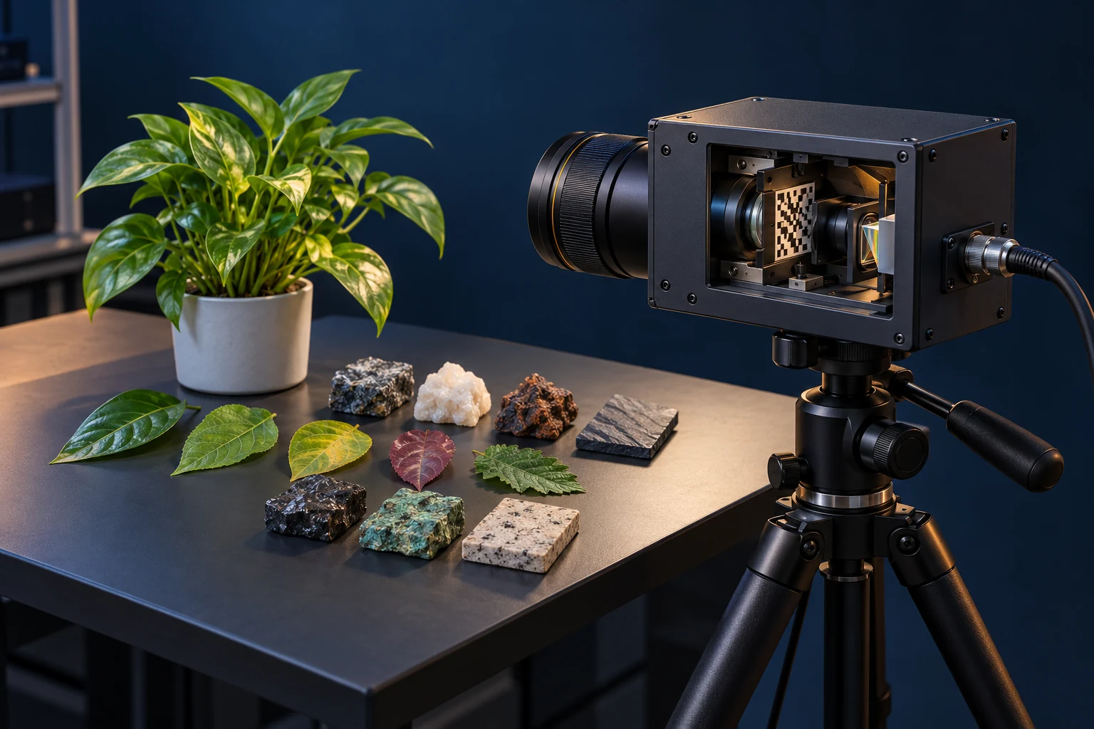
A spectral-scanning arrangement can place a tunable filter in front of an area camera and record a sequence of band images. The filter selects a passband, an image is acquired, and the passband changes for the next image. An original SWIR system-design paper describes an arrangement combining an InGaAs camera, lens and liquid crystal tunable filter, or LCTF. 6
This approach is convenient when a stationary scene and selectable wavelengths are useful. Its main timing limitation is that bands are acquired at different moments. If a leaf moves or illumination changes between bands, a spectrum assembled at one pixel may represent several physical conditions. Image registration can help with alignment but cannot guarantee that the sample itself remained unchanged.
Plan settling time, exposure and wavelength-dependent transmission together. Thorlabs' documented LCTF series includes device-specific switching-time calibration. Check the actual filter's bandwidth, throughput and operating range. These archived documents explain a mechanism; they are not a claim that a particular archived product is currently available. 7
Match the detector and light to the wavelength range
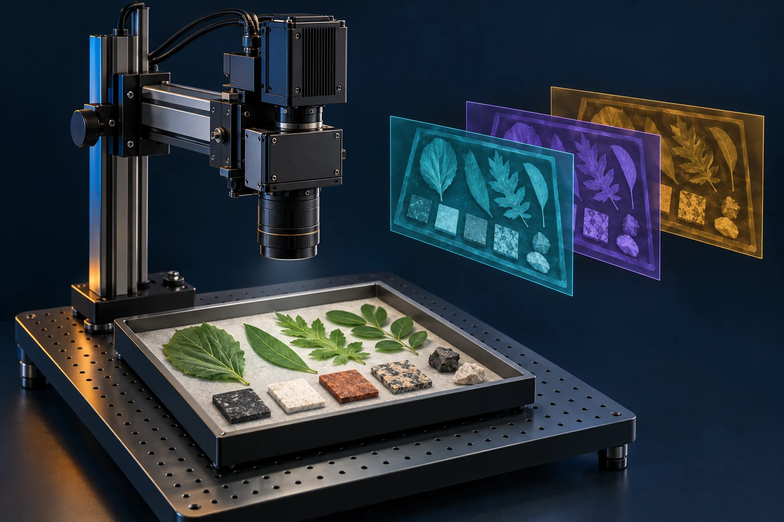
The detector must be sensitive across the wavelengths needed for the task. Silicon is widely used for visible and shorter near-infrared measurements. InGaAs supports longer wavelengths; Hamamatsu distinguishes standard InGaAs sensitivity around 900–1700 nm from extended variants reaching approximately 2500 nm. The exact response depends on the detector, so use its response curve rather than assuming a material name guarantees a particular range. 8
Illumination must also deliver enough light in those bands. A lamp that looks bright to the eye may provide little signal where the analysis needs it. Check the measured response across the full range and avoid exposure choices that saturate strong bands while leaving weak bands near the noise floor.
Longer exposures can collect more photons but increase motion blur or acquisition time. Cooling, detector response, dark signal and optical throughput affect the usable result. Compare actual signal quality under the intended scene and speed instead of assuming the widest wavelength range is automatically preferable.
Capture references and inspect failure modes
A useful calibration plan includes dark measurements, a suitable known reflectance reference, wavelength checks and a geometric check. Capture references under conditions matched to the sample, including exposure, gain, illumination and geometry. Pillay, Hardeberg and George's acquisition workflow explains how these conditions influence quantitative reflectance imaging and spatial correction. 9
Dark subtraction addresses a measured baseline. Reference normalisation can compensate for illumination and instrument response under the assumed arrangement. Wavelength calibration establishes where each band lies spectrally. Geometric calibration and registration address where measurements lie spatially. These operations solve different problems; no single reference image establishes all of them.
Inspect data before applying a model. Saturation, low-signal regions, shadow, reflections, poor focus and line discontinuities are acquisition problems that can resemble material differences. Where conditions vary over time, repeat references or monitor the variation. Retain acquisition parameters and reference data alongside the cube so processing can be reproduced.
- Confirm useful signal across the required wavelength range.
- Match line spacing to motion and the intended spatial sampling.
- Check references, saturation and geometry before material analysis.
- Test repeatability with separate acquisitions under realistic conditions.
Sources: [9]
Run a scan-planning calculation
The standard-library Python example calculates line spacing and movement during exposure for the illustrative pushbroom setup above. It requires Python 3. Use consistent units: speed in mm/s, rate in lines/s and exposure in seconds. The calculation is exact for constant translational motion under those assumptions.
The interactive calculator changes line rate for a fixed 1000-line synthetic scan. Increasing line rate reduces ideal acquisition time. In an actual moving setup it also changes line spacing when speed is fixed. Exposure remains a separate acquisition setting: shortening it reduces movement during exposure, but may weaken the signal. The camera timing, readout limits and measured image quality determine the practical choice.
Sources: [1]
Run the example
Prerequisite: Python 3. Examples use synthetic inputs to explain the calculation. Save the snippet as example.py and run python3 example.py.
# Illustrative constant-speed pushbroom setup.
speed_mm_s = 100.0
line_rate_hz = 200.0
exposure_s = 0.002

line_spacing_mm = speed_mm_s / line_rate_hz
movement_mm = speed_mm_s * exposure_s
line_period_s = 1.0 / line_rate_hz

print(f'Line spacing: {line_spacing_mm:.3f} mm')
print(f'Movement during exposure: {movement_mm:.3f} mm')
print(f'Line period: {1000 * line_period_s:.1f} ms')
print(f'Exposure within line period: {exposure_s <= line_period_s}')
Verified output
Line spacing: 0.500 mm
Movement during exposure: 0.200 mm
Line period: 5.0 ms
Exposure within line period: True
Frequently asked questions
Does a pushbroom camera need a moving sample?
It needs relative motion to build the second spatial dimension. The sample, camera or viewing direction can move, depending on the system.
Are AVIRIS and AVIRIS-NG the same scan type?
No. The classic AVIRIS guide describes a whiskbroom scanner, while NASA identifies AVIRIS-NG as a pushbroom instrument.
Does snapshot mean there is no motion blur?
No. Motion during a finite exposure can still blur the data. Snapshot acquisition reduces the need to assemble measurements taken at different times.
Why can tunable-filter spectra be inconsistent?
Bands are captured at different times. Movement or illumination changes can make a pixel's assembled spectrum combine different scene conditions.
Can a white reference replace every calibration?
No. Reference normalisation, wavelength calibration and geometric calibration address different measurement properties.
What limits usable acquisition speed?
Exposure, readout, signal level, movement and the required spatial sampling interact. Verify performance with the actual scene and complete acquisition setup.
References and further reading
- Resonon: Benchtop line-scan system overview
- Johnson and Green: AVIRIS user's guide
- NASA JPL: AVIRIS-NG flight planning
- Deng et al. (2018): Snapshot imaging via spectral basis multiplexing
- Gao et al. (2010): Snapshot image mapping spectrometer
- LCTF-based SWIR imaging system: Design and integration
- Thorlabs: Liquid crystal tunable bandpass filter documentation
- Hamamatsu: NIR and SWIR detector questions
- Pillay, Hardeberg and George (2019): Acquisition and calibration workflows
- NASA JPL: AVIRIS-NG instrument overview